Chapter 7 An Illustrative Example of Travel Cost Methods: The Poisson Model and Applications for Natural Resource Management
Author: James Fogarty
First Release: 31 March 2025
7.1 Before you get started
The Travel Cost Method (TCM) is survey method that is widely used to provide lower bound estimates of the value of recreation sites. There are two types of Travel Cost demand model. Single site models and multi-site (multi-attribute) models. Each model type has a different strength.
Single site models estimate trip demand using a Poisson regression model, and then estimate consumer surplus from the demand equation. The price of a trip is the expenditure incurred, including the opportunity cost of travel time to reach. When the objective is to estimate the total recreation value of a site, single site models are the preferred method. The total value of a site might need to be estimated because the site has to be closed due to a pollution event (eg oil spill), or a lack of funding to keep the site open (budget cuts at National Parks) and an estimate of the loss in value due to the closure is required.
Multi-site (multi-attribute) models are based on trip utility, and the main method of estimation for this type of model is the mixed (random parameter) logit model. This type of model is preferred when the objective is to estimate the value of different attributes at a recreation site or sites. Typically this type of model is called a Random Utility Model. Here the decision to visit a park depending on the cost of getting to the park, and the recreation amenity combination available at the park. Understanding the value of different park attributes allows park managers to plan investments in park infrastructure that provide the greatest value, for example do park users value improved toilet facilities highly, or would they prefer additional walking trails, or overnight accommodation options.
The focus of this guide is the Poisson regression model, and how the model can be used to obtain value estimates for individual recreation sites. This guide provides a short review of the Poisson model, and then presents examples of the TCM implemented in two contexts: off-site sampling, which matches most closely to the theory assumptions of the Poisson model, but is often not the most practical approach to implement, and on-site sampling, which is easier to implement, but requires some data adjustments to be consistent with the theory assumptions of the Poisson model. Fortunately the adjustments for on-site sampling are easy to implement, and so it is possible to use a method that is relatively cost effective to implement and still obtain valid estimates of site value. Additionally, the guide assumes some familiarity with the R platform for statistics.
7.2 Introduction to count data models
With count data it is possible to use the standard linear model estimation framework and in many cases still obtain results that are reasonable, but to use such an approach is not consistent with the underlying Data Generating Process (DGP). For example, when using the lm() function in R it is assumed that the dependent variable can take values from negative \(\infty\) to positive \(\infty\). For count data values can only non-negative integers, hence the DGP assumed with a linear model does not match the DGP for count data.
As a practical matter, the larger the expected number of observed cases (ie the sample mean of the dependent variable is far from zero), the closer the OLS assumptions are to being true. But if the expected number of counts is small, the OLS option is a bad modelling approach to follow. So, the OLS framework will be OK in some instances and not OK in other circumstances, but the Poisson model will always be valid for count data. As such, it makes sense to use the Poisson model as the default approach for count data.
This example uses the AER package, which will also load a number of other packages.
7.2.1 Typical count data context
The following example is calibrated to Western Australian Fisheries data, and is representative of a count data modelling process.
sharks <- data.frame(count = c(1, 0, 2, 0, 1, 2, 1, 0, 1, 4, 1, 2, 0, 2,
    2, 3, 3, 5), pop = c(862952, 879156, 894857, 909520, 923874, 937584,
    952185, 962119, 973093, 984462, 998434, 1016014, 1044436, 1076806, 1110812,
    1136781, 1168359, 1205182), time = c(seq(from = 2005, to = 2022, by = 1)))
In the data set the variables are:
- Count = number of (great white) shark attacks in the year (can only be non-negative)
- Time = index of the years ( this is the trend through time)
- Pop = WA metro population (more people in Perth = more people at the beach more people exposed to shark attack risk
And we can see the structure of these variables as follows:
## 'data.frame':    18 obs. of  3 variables:
##  $ count: num  1 0 2 0 1 2 1 0 1 4 ...
##  $ pop  : num  862952 879156 894857 909520 923874 ...
##  $ time : num  2005 2006 2007 2008 2009 ...
A visual inspection of the data is always an important step:
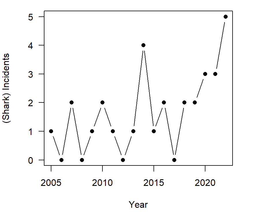
Figure 7.1: The basic data structure
From the plot we can see that the dependent variable only takes non-negative integer values. This makes the standard linear model inappropriate, from a theory perspective
The pattern of attacks through time also looks like it might follow a multiplicative process. Ignoring that the issue of only non-negative integers for the dependent variable, if there are no zero values, a multiplicative process can be modeled using the lm function as \(log(y_{i})=b_{0}+b_{1}x_{i}+e_{i}\). Log zero is not defined, and so if there are zero values a lm model can not be used as an approximation. As there are years with zero values the shark incident data, a model of the form \(log(y_{i})=b_{0}+b_{1}x_{i}+e_{i}\) can not be estimated.
To solve the log zero undefined problem, staff in the Department of Fisheries pooled the data into 24 month periods (there was no two year period without an incident) rather than annual 12 month time periods. This is not a good idea. Pooling time periods halves the sample size, and so unnecessarily increases the chance of a Type-II error. More importantly, we have a specific model for this type of data and so pooling is just not necessary.
A linear model as a comparison case
Although a \(log(Y)\) model can not be estimated, a linear model to the data of the form: \(y_{i}=b_{0}+b_{1}x_{i}+e_{i}\) can be estimated. The model will under predict incidents at the tails of the data (start and end years of the data); over predict incidents in the middle years of the data; and also may predict negative incidents, which is not possible. So this is not a good model to fit, but it is used as a benchmark comparison.
##
## t test of coefficients:
##
##               Estimate Std. Error t value Pr(>|t|)
## (Intercept) -318.33230  106.68467  -2.984  0.00877 **
## time           0.15893    0.05298   2.999  0.00849 **
## ---
## Signif. codes:  0 '***' 0.001 '**' 0.01 '*' 0.05 '.' 0.1 ' ' 1
The lm model says that we expect the number of incidents to increase by around 0.16 each year, and the annual increase is statistically significant. We can also subject the model to the standard range of diagnostic tests:
- reset functional form test
- bp heteroskedasticty test, and
- (because it is a time series model) bg autocorrelation test.
##
##  RESET test
##
## data:  lm1
## RESET = 2.023, df1 = 2, df2 = 14, p-value = 0.169##
## studentized Breusch-Pagan test
##
## data: lm1
## BP = 0.6808, df = 1, p-value = 0.409##
## Breusch-Godfrey test for serial correlation of order up to 1
##
## data: lm1
## LM test = 0.4455, df = 1, p-value = 0.504In this instance the lm model passes all the diagnostic tests. But recall that when the sample size is small, diagnostic tests have low power to detect deviations from the model assumption. The model also really pushes the assumption of a Y as a continuous variable. Shark attacks can only come in whole numbers and the expected number of incidents in any given year is low. This suggests a count data type model.
Note that a log-linear model can not be estimated, as th log of zero is undefined. Historically people suggested adding one to all the values so that the model could be estimated. There is now much research that demonstrates that the log(Y+1) model is, in general, not appropriate. A model of the form \(y_{i}=b_{0}+b_{1}x_{i}^{3}+e_{i}\) could be a plausible fit to the data and can be estimated, but here the point is to introduce the glm model rather than exploit all the possible variation available for a lm model.
The Poisson model motivation
There are ways to motivate the poisson regression model. One possible motivation is as follows. Say, we want to estimate a relationship as follows: \(log(y_{i})=X_{i}b\), which is to say that average expected value of log \(y_{i}\) can be predicted by \(X_{i}b\). Now, assume we have some zero values such that it is not possible to take the log of some \(y_{i}\).
If we undo the log transformation on the \(y_{i}\), and apply the same transformation to the \(X_{i}b\), we get the expression \(y_{i}=exp(X_{i}b)\). So the model is just the log-linear model expressed in a different format, and with a different assumption of the error term. It is fine to think of the log-linear model and Poisson model as different ways of estimating the same relationship.
In R, the Poisson model requires only a slight extension to the lm() model notation, with only one additional parameter setting, which is the family setting, and then changing lm() to glm(). The general form of the Poisson regression model in R is: my.glm <- glm(Y ~ X, data=my.data, family=poisson()), and the specific form for the shark incident data is:
##
## z test of coefficients:
##
##               Estimate Std. Error z value Pr(>|z|)
## (Intercept) -201.88005   76.72294  -2.631  0.00851 **
## time           0.10045    0.03806   2.640  0.00830 **
## ---
## Signif. codes:  0 '***' 0.001 '**' 0.01 '*' 0.05 '.' 0.1 ' ' 1
The model output for the shark data says that for a one unit increase in time (one year) there is an increase in the log count of shark attacks of 0.100, and the increase is statistically significant.
We can compare the predicted values from the two models as follows:
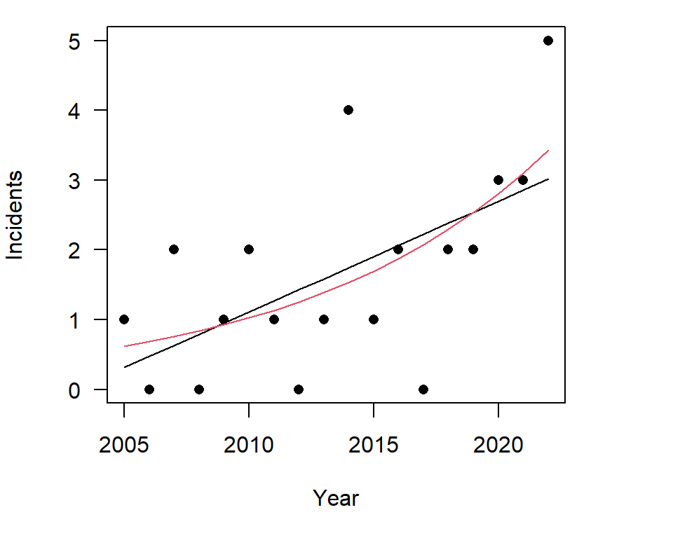
Figure 7.2: The basic data structure
The curve of the poisson model is what we expect with a growth type relationship, but how well does our model fit?
For the Poisson model a pseudo R-squared can be calculated as the difference between the fit of a model with an intercept only and the fit of the current model to come up with a measure of fit. There are also other options for calculating a pseudo R-squared value.
In practice the pseudo R-squared is obtained as follows:
## [1] 0.3194557.2.2 Overdispersion issues
There are two common model assumption violations when estimating the standard Poisson model. The first is that the assumption that the mean equals the variance generally does not hold. The second issue is that are often more zero observed in the data than is the case for the theoretical distribution.
There are several approaches to deal with these problems. In general, to resolve the problem of the mean not equal to the variance people use either: the negative binomial model; the quasi- poisson model; or robust standard errors. All three options result in very similar empirical results.
With poisson models the issue of ‘over-dispersion’ is conceptually similar to the issue of heteroskedasticty (covered in the hedonic model chapter) in that the point estimates remain unbiased and consistent, but the standard errors, and hence hypothesis testing will be wrong. Due to this similarity. Similar to the hedonic chapter, here the focus is on the robust standard error correction approach.
To address the issue of extra zeros, relative to theoretical expectations, zero inflated models are used. A zero inflation model is appropriate when there is a two-part process for the DGP that results in extra zeros, relative to what would be expected from just a count data process. For example, say you survey people at a recreation site and ask them how many fish they caught. Here, there is a two-part process. First, there is the decision to fish or not, and many people will not fish (a zero-one DGP). Next, there is the number of fish caught (a count model DGP). Because many people choose not to fish, there will be many extra zeros, relative to expectations for a pure count data model. The zero-inflated model combines a logit model for the decision to fish or not part and a count data model for the how many fish were caught part.
Most TCM scenarios do not require a zero-inflation model.
We can test for over dispersion using a test from the AER package as follows.
##
##  Overdispersion test
##
## data:  fit1
## z = -1.138, p-value = 0.872
## alternative hypothesis: true dispersion is greater than 1
## sample estimates:
## dispersion
##   0.723579
For this we test just look at the p-value. With a low p-value we reject the null of equality of mean and variance. Here the test p-value > 0.05 so it is reasonable to assume that mean equals he variance assumption is valid and that it is possible to proceed with normal hypothesis testing..
Note that if we had failed the overdispersion test we could use the robust covariance matrix approach to obtain valid standard errors for hypothesis testing.
##
## z test of coefficients:
##
##              Estimate Std. Error z value Pr(>|z|)
## (Intercept) -201.8801    70.9996  -2.843  0.00446 **
## time           0.1004     0.0352   2.854  0.00432 **
## ---
## Signif. codes:  0 '***' 0.001 '**' 0.01 '*' 0.05 '.' 0.1 ' ' 1
Note: the negative binomial model allows the mean and the variance to be different. The negative binomial model is not as common in the TCM literature as the robust variance approach, and the negative binomial optimiser in the MASS package can be difficult to work with.The quasipoisson option is available in R as: my.glm <- glm(Y ~ X, data=my.data, family=quasipoisson()), but it is not common to see this approach in the TCM literature. The robust option is both valid and commonly used, so we can proceed with confidence with this method.
7.2.3 The incident rate
Poisson model results involving a time variable are often described not by the raw model coefficients, but by the Incident Rate value. The incident rate is found by taking the anti-log of the model point estimate, subtracting one, and multiplying by 100.
## (Intercept)        time
## 2.11158e-88 1.10567e+00
The transformed point estimate of the Time variable is interpreted as follows: We say that there is a (1.11 - 1.0) x 100 = 11 percent increase in the incident rate each year. We can then get the confidence interval around the Incident rate as:
##                    2.5 %      97.5 %
## (Intercept) 1.30251e-156 4.35575e-25
## time         1.02851e+00 1.19521e+00
Or if we want to put it all together we can use:
##                estimate        2.5 %      97.5 %
## (Intercept) 2.11158e-88 1.30251e-156 4.35575e-25
## time        1.10567e+00  1.02851e+00 1.19521e+00
You can see from this result that the CI range for the incident rate version of the effect of time is between around three percent and 20 percent, so it is actually quite a wide range.
Now, let’s look at some specific predicted values and see if we can understand what is going on. We can calculate predicted values for different time periods as follows.
##       1
## 0.62171## 1
## 0.687406## 1
## 0.760044So we have as our predicted counts at time 1, 2 and 3 as shown above
We then have the change in the predicted counts across time periods as:
predict(fit1, data.frame(time =2006), type="response" ) -
  predict(fit1, data.frame(time =2005), type="response" )
## 1
## 0.065696predict(fit1, data.frame(time =2007), type="response" ) -
predict(fit1, data.frame(time =2006), type="response" )## 1
## 0.072638predict(fit1, data.frame(time =2021), type="response" ) -
predict(fit1, data.frame(time =2020), type="response" )## 1
## 0.296429Note that the change in the predicted values is increasing. This can be seen by plotting the change in the marginal value.
##        1        2        3        4        5        6        7        8
## 0.621710 0.687406 0.760044 0.840358 0.929158 1.027342 1.135901 1.255932
##        9       10       11       12       13       14       15       16
## 1.388646 1.535384 1.697627 1.877015 2.075359 2.294661 2.537138 2.805236
##       17       18
## 3.101665 3.429417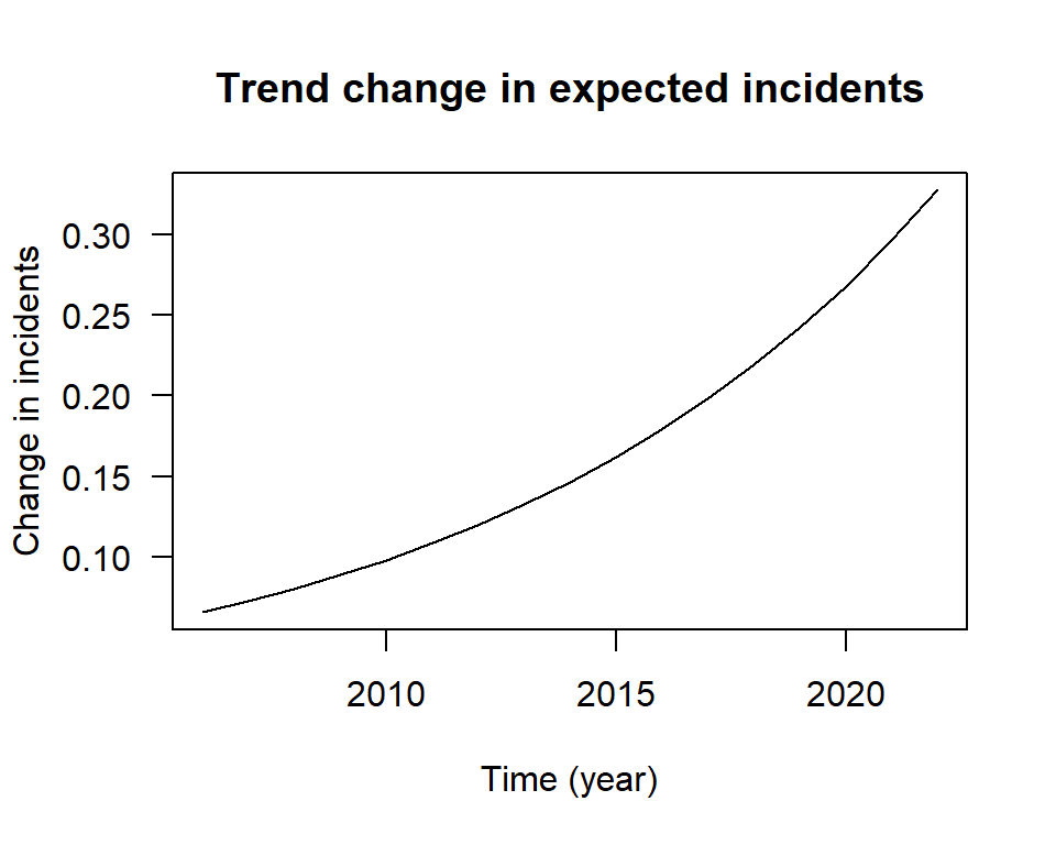
Figure 7.3: The increasing marginal effect
7.2.4 The offest in the Poisson model
We control for the effect of population growth with an offset. We could just add population as an effect to be estimated to the model. However, we are really combining different types of information here. Rather than estimate the effect of population growth we want to control for the the additional effective exposure due to population growth. We know what was actually happening with population, so we control for this effect. In this case it would be even better to control for the growth in the number of surfers in the water, but this information is not available.
To illustrate the difference, let us first add population to the model as a co-variate
##
## Call:
## glm(formula = count ~ time + log(pop), family = poisson(), data = sharks)
##
## Coefficients:
##             Estimate Std. Error z value Pr(>|z|)
## (Intercept)   5.9553   288.7631    0.02     0.98
## time         -0.0576     0.2158   -0.27     0.79
## log(pop)      7.9972    10.7781    0.74     0.46
##
## (Dispersion parameter for poisson family taken to be 1)
##
##     Null deviance: 23.581  on 17  degrees of freedom
## Residual deviance: 15.489  on 15  degrees of freedom
## AIC: 57.29
##
## Number of Fisher Scoring iterations: 5
Note that when we add the population co-variate to the model both population and the time variable are not statistically different from zero. This is because population and the time variable are correlated. To control for the impact of higher population through time, rather than estimate the effect of population, we use an offset. The way we specify this in the model is as follows.
Technically, as we have a different model we want to again check the dispersion assumption, which we do as follows.
##
##  Overdispersion test
##
## data:  fit3
## z = -1.133, p-value = 0.871
## alternative hypothesis: true dispersion is greater than 1
## sample estimates:
## dispersion
##   0.721861
As the test results suggests no major issue with overdispersion, we look at the summary() output.
##
## Call:
## glm(formula = count ~ time + offset(log(pop)), family = poisson(),
##     data = sharks)
##
## Coefficients:
##              Estimate Std. Error z value Pr(>|z|)
## (Intercept) -175.8403    76.1457   -2.31    0.021 *
## time           0.0807     0.0378    2.14    0.033 *
## ---
## Signif. codes:  0 '***' 0.001 '**' 0.01 '*' 0.05 '.' 0.1 ' ' 1
##
## (Dispersion parameter for poisson family taken to be 1)
##
##     Null deviance: 20.791  on 17  degrees of freedom
## Residual deviance: 15.916  on 16  degrees of freedom
## AIC: 55.71
##
## Number of Fisher Scoring iterations: 5
The results says that for a one unit increase in time (one year) controlling for the effect of population growth, there is an increase in the log count of shark attacks of 0.0807, and this effect is statistically significant. So, controlling for the growth in the population, the observed effect (trend) is still statistically significant, but the increase is less than without the offset. Some of the increase is due to more people at the beach and some is due to a genuine increase.
We can also get the incident rate measure:
## (Intercept)        time
## 4.30075e-77 1.08400e+00
This says that for each year that passes we expect the count to increase by 1.08, and so we can say that each year we expect an 8 percent increase in the incident rate.
Finally, we can compare our different models as follows:
par(mfrow = c(1, 1), mar = c(5, 4, 1, 4))
plot(count ~ time, ylab = "Shark incidents", pch = 16, col = "grey", las = 1,
    xlab = " Time (years)", data = sharks)
lines(seq(from = 2005, to = 2022, by = 1), predict(lm1, type = "response"),
    col = 1)
lines(seq(from = 2005, to = 2022, by = 1), predict(fit1, type = "response"),
    col = 2)
lines(seq(from = 2005, to = 2022, by = 1), predict(fit3, type = "response"),
    col = 3)

legend("topleft", legend = c("Observations", "Linear model", "Poission model",
    "Poission with pop control"), lty = c(NA, 1, 1, 1), pch = c(16, NA, NA,
    NA), col = c("grey", 1, 2, 3), bty = "n", cex = 0.8)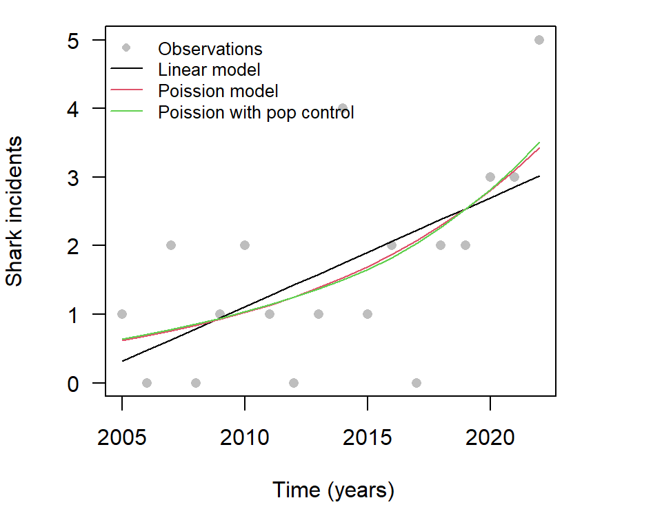
Figure 7.4: Comparison of models
Note that once we control for population growth we had a smaller growth rate in incidents. Including a control for population is an important factor to consider when using this type of model.
7.3 The travel cost model
7.3.1 An overview
The (single site) Travel Cost Model (TCM) seeks to estimate the value of parks based on the cost of time it takes to get to the park. Because trips to a park can not be negative, and people make one trip, two trips, etc., a count data model is appropriate to estimate the demand curve for a park.
The general steps in the process are as follows:
- Step 1 Define the site to be valued
- Step 2 Define the recreation uses and the season
- Step 3 Develop a sampling strategy
- Step 4 Specify the model
- Step 5 Decide on the treatment of multiple purpose trips
- Step 6 Design and implement the survey
- Step 7 Measure trip cost
- Step 8 Estimate the model
- Step 9 Calculate access value from consumer surplus estimate
Consumer Surplus is defined as the the area below the demand curve and above the price paid to get to the park. This area represents the difference between the use value generated from the park and the cost people incurred to access the park. Consumer Surplus is a widely used metric to value net benefits.
If we increase the cost of accessing the park, by say increasing the gate fee, the consumer surplus falls. If we increase the quality of the park, due, for example, to making some improvements to the facilities at the park, then for any given price, there is a increase in trips to the park. The demand curve shifts to the right and Consumer Surplus increases.
The research objective is to calculate Consumer Surplus, and fortunately, with the Poisson regression model, the Consumer Surplus calculation is simple.
7.3.2 The questionaire
The TCM is a survey based method. The survey questionnaire usually has several components. An example could be as follows.
- Introduction
- Introductory remarks
- Use of the site of interest (e.g. did you fish)
- Lifestyle questions (e.g. did you drive an SUV to the site)
- Valuation section
- Number of visits
- Site quality
- Travel costs
- Substitutes
- Demographic information
- Age
- Income
- Education
- Gender
7.3.3 Travel cost model
The actual model estimated takes the following form:
No. of visits = travel costs + site quality + substitute options + demographic attributes
## 'data.frame':    659 obs. of  6 variables:
##  $ ID    : int  1 2 3 4 5 6 7 8 9 10 ...
##  $ trips : int  0 0 0 0 0 0 0 0 0 0 ...
##  $ ski   : Factor w/ 2 levels "no","yes": 2 1 2 1 2 2 1 2 1 1 ...
##  $ income: int  4 9 5 2 3 5 1 5 2 3 ...
##  $ costS : num  68.6 70.9 59.5 13.8 34 ...
## $ costH : num 76.8 84.8 72.1 23.7 34.5 ...## Min. 1st Qu. Median Mean 3rd Qu. Max.
## 0.00 0.00 0.00 2.24 2.00 88.00Note the distribution of trips includes zeros. This means that the survey is an off-site survey. For an off-site survey, in general, most people will not have visited the park. There is also one respondent that reported visiting the park 88 times. This could be a data entry error. Checking the data, the entry was found to be correct but it is important to check.
- Description of variables
- ID = A record of respondents
- trips = Number of recreational boating trips taken to Lake Sommerville
- ski = Factor (Dummy) variable if water-skiing at the Lake
- income = Annual household income of the respondent (in ’0,000 USD).
- costS = Expenditure when visiting Lake Somerville (in USD) main interest
- costH = Expenditure when visiting Lake Houston (in USD) = substitute lake
The model estimated is that the trips to Lake Somerville depend on the cost of getting to Lake Somerville, income, the value obtained from activities available at the lake, which here is whether or nor we ski, and the cost of getting to an alternate destination. And we test for overdispersion.
##
##  Overdispersion test
##
## data:  rd2
## z = 4.278, p-value = 9.42e-06
## alternative hypothesis: true dispersion is greater than 1
## sample estimates:
## dispersion
##    7.48835
As we fail the overdispersion test we obtain robust SE values for inference as follows:
##
## z test of coefficients:
##
##             Estimate Std. Error z value Pr(>|z|)
## (Intercept)  1.26305    0.32331   3.907 9.36e-05 ***
## costS       -0.06017    0.01692  -3.556 0.000376 ***
## costH        0.05057    0.01382   3.659 0.000253 ***
## skiyes       0.66879    0.30935   2.162 0.030627 *
## income      -0.08760    0.05029  -1.742 0.081504 .
## ---
## Signif. codes: 0 '***' 0.001 '**' 0.01 '*' 0.05 '.' 0.1 ' ' 1## [1] 0.316636The results say:
- As the cost of getting to Lake Sommerville increases, people make fewer trips to Lake Sommerville
- As the cost of getting to Lake Houston increases, people make more trips to Lake Sommerville (ie the two lakes are substitute products, which makes sense)
- People that ski make more trips to Lake Sommerville than people that do not water ski
- As income goes up, people make fewer trips to Lake Sommerville, but the effect is only marginally statistically significant.
The main research focus is to obtain an estimate of the value of the site (Lake Sommerville) so that policy makers have some understanding of how important the site is.
The predicted average consumer surplus is found as one divided by the estimate on the cost parameter, as so here can be found as:
# average surplus
deltaMethod(rd2, "1/-b1" ,  vcov. = vcovHC(rd2), parameterNames= paste("b", 0:3, sep=""))
## Estimate SE 2.5 % 97.5 %
## 1/-b1 16.619 4.673 7.459 25.78So, we can say that $16.62 per trip is the average consumer surplus.
Now, say that from independent entry records at the site we know that 168,567 people visited Lake Sommerville during the year. We combine the visitor information with our surplus estimate to get an annual value for the park. So we have 168,567 \(/time\) $16.62 = $2,801,584.
This means that the site has an annual recreation value of $2.8M. There are potentially many other values associated with the site, but we have captured something that can be used in policy evaluation. We might think of it as a lower bound value.
We then convert this annual value into a net present value. Assuming no population change and no site characteristic change, We can divide through by the discount rate to get the NPV. Typically, because no-one can agree, you report a range of values, and typical values for the real discount rate are 3%, 5%, and 7%. The formula to use is annual total value divided by discount rate. So, in this case if we divide through by 5%, we get a NPV for the Park of $56.0M.
This approach has not captured all of the value of the park. It is just a start, but it might help change perceptions in the policy world if we can start to show these values. It might be all we need to get policy makers to engage more fully with the value of recreation sites.
7.4 Onsite survey
An onsite Travel Cost survey is a cost effective way to obtain data. The main issue with on-site surveys is that regular visitors are over sampled and the minimum value observed is one. To be part of the survey the person has to be at the site. This example is based on the data available at: https://www.env-econ.net/2008/10/travel-cost-met.html
## 'data.frame':    151 obs. of  6 variables:
##  $ casenum: int  7 20 21 28 29 38 41 47 48 49 ...
##  $ income2: num  87.5 87.5 150 87.5 125 87.5 20 125 125 125 ...
##  $ TCWB   : num  1121 657 975 754 915 ...
##  $ TCOB   : num  887 434 676 525 638 ...
##  $ rating : int  4 4 4 4 4 5 5 4 3 5 ...
## $ trips : int 4 4 1 1 4 7 1 1 1 3 ...## Min. 1st Qu. Median Mean 3rd Qu. Max.
## 1.0 1.0 3.0 11.4 8.5 80.0variable descriptions casenum = index for survey responses income2 = household income in thousands TCWB = travel cost to Wrightsville Beach (including time costs) TCOB = travel cost to the Outer Banks, a substitute (including time costs) rating = a subjective beach quality variable trips = day trips to Wrightsville Beach, NC, the dependent variable
First, let us estimate consumer surplus, ignoring the oversampling and endogenous stratification bias and proceed as we would for an off-site model.
##
##  Overdispersion test
##
## data:  glm.b1
## z = 4.686, p-value = 1.39e-06
## alternative hypothesis: true dispersion is greater than 1
## sample estimates:
## dispersion
##    13.6038
As the model fails the overdispersion test the model results are obtained as:
glm.b1 <-glm(trips~income2 +TCWB +TCOB +rating, data=BD, family=poisson() )
coeftest(glm.b1, vcovHC(glm.b1))
##
## z test of coefficients:
##
## Estimate Std. Error z value Pr(>|z|)
## (Intercept) 1.278582 0.687875 1.859 0.0631 .
## income2 -0.013867 0.003092 -4.485 7.31e-06 ***
## TCWB -0.008903 0.001571 -5.667 1.45e-08 ***
## TCOB 0.006388 0.001608 3.972 7.12e-05 ***
## rating 0.394878 0.177586 2.224 0.0262 *
## ---
## Signif. codes: 0 '***' 0.001 '**' 0.01 '*' 0.05 '.' 0.1 ' ' 1## [1] 0.578397The results say that as income increases trips to the beach decrease, as the cost of visiting the beach increases, trips decrease, as the cost of visiting the substitute beach increases, trips to the target beach increase, the higher the subjective rating of the beach the more trips are made.
##       Estimate     SE  2.5 % 97.5 %
## 1/-b2   112.32  19.82  73.48  151.2
To correct for over sampling beach goers that attend the beach regularly, and so have a high value, all that is needed is to subtract one from the dependent variable. With this adjustment the consumer surplus estimate can be calculated using the same formula as previously used. This adjustment is implemented in R as follows:
glm.b2 <-glm(trips-1~income2 +TCWB +TCOB +rating, data=BD, family=poisson() )
dispersiontest(glm.b2)
##
## Overdispersion test
##
## data: glm.b2
## z = 3.324, p-value = 0.000444
## alternative hypothesis: true dispersion is greater than 1
## sample estimates:
## dispersion
## 23.4556##
## z test of coefficients:
##
## Estimate Std. Error z value Pr(>|z|)
## (Intercept) 1.175286 0.809470 1.452 0.146524
## income2 -0.015232 0.004046 -3.765 0.000166 ***
## TCWB -0.011106 0.001908 -5.821 5.86e-09 ***
## TCOB 0.007123 0.002046 3.481 0.000499 ***
## rating 0.408830 0.202044 2.023 0.043024 *
## ---
## Signif. codes: 0 '***' 0.001 '**' 0.01 '*' 0.05 '.' 0.1 ' ' 1## [1] 0.6011## Estimate SE 2.5 % 97.5 %
## 1/-b2 90.04 12.74 65.08 115Qualitatively, the results between the two model specifications are similar, but the estimate of consumer surplus falls from $112 per visit to $90 per visit. So, failing to account for the bias introduced by on-site sampling results, in this case, in an over statement of the per person per visit central consumer surplus estimate of approximately \(log(112) - log(90) \times 100 = 22\%\), which is a material overstatement of the benefit.