Chapter 2 A Brief Example of Discrete Choice Experiments using the support.CEs and apollo Packages
Author: Hideo Aizaki
Latest Revision: 9 March 2021 (First Release: 29 August 2019)
2.1 Before you get started
This tutorial, which is a revised version of Aizaki (2012, sec. 4.1), presents the process of discrete choice experiments (DCEs) using R (R Core Team 2021a) combained with the support.CEs (Aizaki 2012) and apollo (Hess and Palma 2019, 2021) packages. The apollo package, available from the Comprehensive R Archive Network (CRAN), enables the user to estimate various discrete choice models.
Please refer to Aizaki (2012) and Aizaki, Nakatani, and Sato (2014) for detailed explanation on the support.CEs package, and visit www.ApolloChoiceModelling.com for that on the apollo package, including the full user manual.
2.2 Outline of the example
We explain how to use the packages on the basis of a hypothetical DCE study about consumers’ preferences for an agricultural product (for details, see Aizaki (2012, sec. 4.1)). The respondents were asked to select their preferred alternative from two agricultural products and an option “none of these.” The agricultural product alternative consists of three attributes, in which each one has three levels:
- Region of origin: region A, region B, and region C
- Cultivation methods: conventional method, more eco-friendly method, and most eco-friendly method
- Price per piece: $1, $1.1, and $1.2
The responses to the DCE questions were analyzed using a conditional/multinomial logit model with the following systematic components of utility functions:
\[\begin{align} V_1 &= asc + \beta_{Reg\_B} Reg\_B_{1} + \beta_{Reg\_C} Reg\_C_{1} + \beta_{More} More_{1} + \beta_{Most} Most_{1} + \beta_{Price} Price_{1}, \\ V_2 &= asc + \beta_{Reg\_B} Reg\_B_{2} + \beta_{Reg\_C} Reg\_C_{2} + \beta_{More} More_{2} + \beta_{Most} Most_{2} + \beta_{Price} Price_{2}, \\ V_3 &= 0, \end{align}\]
where \(asc\) and \(\beta\)s are coefficients to be estimated; \(Reg\_B\) and \(Reg\_C\) are dummy-coded variables corresponding to region B and region C, respectively; \(More\) and \(Most\) are dummy-coded variables corresponding to more eco-friendly cultivation method and most eco-friendly cultivation method, respectively; and \(Price\) is the price variable.
2.3 Loading packages
Let us load the packages needed for this tutorial into the current R session:
Note that the following line of code is needed to reproduce the results on R 3.6.0 or later:
## Warning in RNGkind(sample.kind = "Rounding"): non-uniform 'Rounding' sampler
## used
2.4 Designing choice sets
Choice sets for the study were created using the mix-and-match method.
The function rotation.design() in the support.CEs package
generates the choice sets according to the attributes and their levels:
des1 <- rotation.design(
   attribute.names = list(
     Region = c("Reg_A", "Reg_B", "Reg_C"),
     Eco    = c("Conv.", "More", "Most"),
     Price  = c("1", "1.1", "1.2")),
   nalternatives = 2,
   nblocks = 1,
   row.renames = FALSE,
   randomize = TRUE,
   seed = 987)
des1
##
## Choice sets:
## alternative 1 in each choice set
## BLOCK QES ALT Region Eco Price
## 1 1 1 1 Reg_B More 1.1
## 8 1 2 1 Reg_B Most 1
## 9 1 3 1 Reg_A Most 1.1
## 6 1 4 1 Reg_A Conv. 1
## 3 1 5 1 Reg_C Most 1.2
## 7 1 6 1 Reg_A More 1.2
## 5 1 7 1 Reg_C Conv. 1.1
## 4 1 8 1 Reg_B Conv. 1.2
## 2 1 9 1 Reg_C More 1
##
## alternative 2 in each choice set
## BLOCK QES ALT Region Eco Price
## 1 1 1 2 Reg_C Most 1.2
## 5 1 2 2 Reg_A More 1.2
## 8 1 3 2 Reg_C Conv. 1.1
## 4 1 4 2 Reg_C More 1
## 3 1 5 2 Reg_A Conv. 1
## 9 1 6 2 Reg_B Conv. 1.2
## 2 1 7 2 Reg_A Most 1.1
## 7 1 8 2 Reg_B Most 1
## 6 1 9 2 Reg_B More 1.1
##
## Candidate design:
## A B C
## 1 2 2 2
## 2 3 2 1
## 3 3 3 3
## 4 2 1 3
## 5 3 1 2
## 6 1 1 1
## 7 1 2 3
## 8 2 3 1
## 9 1 3 2
## class=design, type= oa
##
## Design information:
## number of blocks = 1
## number of questions per block = 9
## number of alternatives per choice set = 2
## number of attributes per alternative = 3The resultant nine choice sets corresponds to nine DCE questions, which were assumed to be assigned to each of the 100 respondents.
2.5 Preparing a dataset for analysis
The responses to the DCE questions are stored in the dataset syn.res1
in the support.CEs package:
## [1] 100 12## ID BLOCK q1 q2 q3 q4 q5 q6 q7 q8 q9 F
## 1 1 1 2 1 2 2 2 1 2 3 1 0
## 2 2 1 1 1 1 1 3 1 3 2 2 1
## 3 3 1 1 2 1 2 2 3 3 3 1 0
## 4 4 1 3 3 1 2 1 1 2 2 1 1
## 5 5 1 3 3 1 1 1 3 2 3 1 1
## 6 6 1 3 1 1 1 3 1 3 3 3 0The dataset contains a variable ID (the respondent identification
number), a variable BLOCK (the block number of choice sets), variables
q1 to q9 (the responses to nine DCE questions), and a variable F
(the respondent’s gender: 1 for female, 0 otherwise).
The choice sets were converted into a design matrix, which was combined
with the dataset to create a dataset for analysis. The function
make.design.matrix() is used to create the design matrix from the
choice sets, while the function make.dataset() is used to merge the
dataset with the design matrix:
desmat1 <- make.design.matrix(
   choice.experiment.design = des1,
   categorical.attributes = c("Region", "Eco"),
   continuous.attributes = c("Price"),
   optout = TRUE,
   unlabeled = TRUE)
dataset1 <- make.dataset(
   respondent.dataset = syn.res1,
   choice.indicators = c("q1", "q2", "q3", "q4", "q5", "q6", "q7", "q8", "q9"),
   design.matrix = desmat1)
The format of the resultant dataset dataset1, in which a row
corresponds to an alternative, differs from that for the apollo
package, in which a row corresponds to a choice set. Therefore,
datasete1 needs to be converted into a dataset with a suitable format
for apollo, using the function reshape() in the stats package:
dataset1r <- reshape(
   dataset1, timevar = "ALT", idvar = "STR",
   v.names = c("RES", "ASC", "Reg_B", "Reg_C", "More", "Most", "Price"),
   drop = "F",
   direction = "wide")
Further, we have to create a variable indicating the responses to the
DCE questions that are in an appropriate format for apollo. The
following R code chunk creates a variable choice:
##    ID BLOCK QES STR RES.1 ASC.1 Reg_B.1 Reg_C.1 More.1 Most.1 Price.1 RES.2
## 1   1     1   1 101 FALSE     1       1       0      1      0     1.1  TRUE
## 4   1     1   2 102  TRUE     1       1       0      0      1     1.0 FALSE
## 7   1     1   3 103 FALSE     1       0       0      0      1     1.1  TRUE
## 10  1     1   4 104 FALSE     1       0       0      0      0     1.0  TRUE
## 13  1     1   5 105 FALSE     1       0       1      0      1     1.2  TRUE
## 16  1     1   6 106  TRUE     1       0       0      1      0     1.2 FALSE
##    ASC.2 Reg_B.2 Reg_C.2 More.2 Most.2 Price.2 RES.3 ASC.3 Reg_B.3 Reg_C.3
## 1      1       0       1      0      1     1.2 FALSE     0       0       0
## 4      1       0       0      1      0     1.2 FALSE     0       0       0
## 7      1       0       1      0      0     1.1 FALSE     0       0       0
## 10     1       0       1      1      0     1.0 FALSE     0       0       0
## 13     1       0       0      0      0     1.0 FALSE     0       0       0
## 16     1       1       0      0      0     1.2 FALSE     0       0       0
##    More.3 Most.3 Price.3 choice
## 1       0      0       0      2
## 4       0      0       0      1
## 7       0      0       0      2
## 10      0      0       0      2
## 13      0      0       0      2
## 16      0      0       0      1
2.6 Preparing an analysis
Before explaining the R code of a conditional logit model analysis using the apollo package, we will outline the analysis scheme using apollo according to Hess and Palma (2019) and the vignette of apollo.
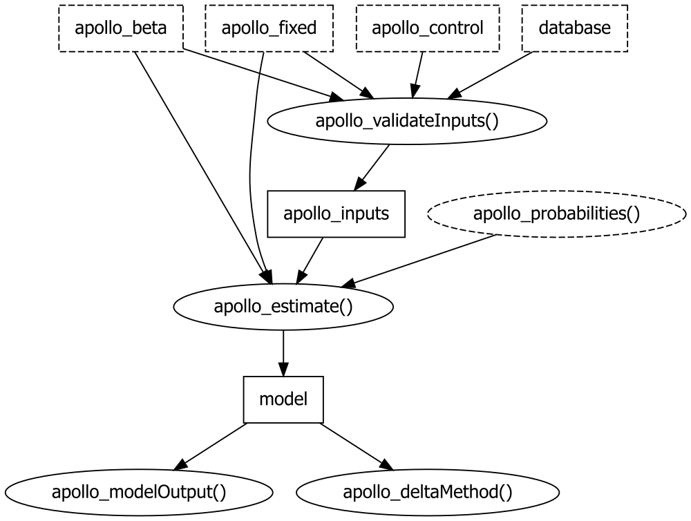
Figure 2.1: A flow for estimating a conditional logit model using apollo
Figure 2.1 shows a flow for implementing a discrete choice model analysis
using apollo in a simple case (i.e., a conditional logit model). In
the flow, rectangles indicate R objects (i.e., a vector, data frame,
and list), while ovals indicate R functions. Solid ovals and
rectangles correspond to functions in apollo and objects created by
these functions, respectively. Dashed oval and rectangles refer to
function and objects that the user is required to create. The core
function apollo_estimate() is used to estimate discrete choice models
and it requires four R object inputs: apollo_beta, apollo_fixed,
apollo_inputs, and apollo_probabilities(). The apollo_inputs
object is created using the function apollo_validateInputs(), whose
inputs are apollo_beta, apollo_fixed, apollo_control, and database.
The apollo_beta is a named vector whose elements are named after
parameters to be estimated, and whose values correspond to the starting
values. The apollo_fixed is a character vector containing parameter
names (similar to those used in apollo_beta) that are fixed when
estimating the model. If the model does not contain any fixed
parameters, NULL is assigned to apollo_fixed.
The apollo_control is a list object containing the
main conditions for the estimation. The database is a data frame
containing variables used in the estimation. The
apollo_probabilities() is a user-defined function, in which
probabilities of selecting alternatives are calculated according to the
discrete choice model defined by the user.
Although the apollo package has various functions for the output,
which is generated from apollo_estimate(), we will use only two:
apollo_modelOutput() and apollo_deltaMethod(). The former one
summarizes the output, while the latter one implements the delta method.
In the example below, the apollo_deltaMethod() will be employed to
calculate the marginal willingness to pays (MWTPs) for non-monetary
attributes and/or their levels.
Let us now go back to the explanation of the R code chunks for estimating the model. The first task for preparing the analysis is to initialize the current session:
The second task is to prepare the inputs, which are apollo_control,
database, apollo_beta, and apollo_fixed, for the function
apollo_validateInputs(). The list object apollo_control consists of
three elements: the name of the model (modelName), its description
(modelDescr), and the name of the respondent identification number
variable (indivID):
apollo_control <- list(
   modelName = "CL_apollo",
   modelDescr = "Consumers' preferences for an agricultural product",
   indivID = "ID"
)
Although our dataset dataset1r has already been created, it is stored
into another object database whose name is mandatory:
According to the systematic components of the utility functions, the
parameter names and starting values of the named vector apollo_beta
are set as:
There are no parameters with fixed values in our model settings,
therefore, the apollo_fixed vector is set to NULL:
These inputs are validated and, afterwards, merged into the list object
apollo_inputs using the function apollo_validateInputs():
## Several observations per individual detected based on the value of ID.
##   Setting panelData in apollo_control set to TRUE.
## All checks on apollo_control completed.
## All checks on database completed.
The final task for the preparation is to define the function
apollo_probabilities(). The following R code chunk is responsible
for this definition, according to the model specification:
apollo_probabilities <- function(apollo_beta, apollo_inputs, functionality = "estimate"){
   apollo_attach(apollo_beta, apollo_inputs)
   on.exit(apollo_detach(apollo_beta, apollo_inputs))

   P <- list()

   V <- list()
   V[['alt1']] = asc + b_RegB*Reg_B.1 + b_RegC*Reg_C.1 + b_More*More.1 + b_Most*Most.1 +
                 b_Price*Price.1
   V[['alt2']] = asc + b_RegB*Reg_B.2 + b_RegC*Reg_C.2 + b_More*More.2 + b_Most*Most.2 +
                 b_Price*Price.2
   V[['alt3']] = 0

   mnl_settings <- list(
     alternatives = c(alt1 = 1, alt2 = 2, alt3 = 3),
     avail        = list(alt1 = 1, alt2 = 1, alt3 = 1),
     choiceVar    = choice,
     V            = V
   )

   P[['model']] <- apollo_mnl(mnl_settings, functionality)
   P <- apollo_panelProd(P, apollo_inputs, functionality)
   P <- apollo_prepareProb(P, apollo_inputs, functionality)

   return(P)
}
Refer to Hess and Palma (2019) for details about the components in
apollo_probabilities().
2.7 Conducting the analysis using apollo
The conditional logit model is estimated with the function
apollo_estimate(). The results are subsequently stored into an object
model in list format:
model <- apollo_estimate(apollo_beta, apollo_fixed, apollo_probabilities, apollo_inputs,
                         estimate_settings = list(writeIter = FALSE))
## Preparing user-defined functions.
##
## Testing likelihood function...
##
## Overview of choices for MNL model component :
## alt1 alt2 alt3
## Times available 900.00 900.00 900.00
## Times chosen 260.00 275.00 365.00
## Percentage chosen overall 28.89 30.56 40.56
## Percentage chosen when available 28.89 30.56 40.56
##
##
## Pre-processing likelihood function...
##
## Testing influence of parameters
## Starting main estimation
##
## BGW using analytic model derivatives supplied by caller...
##
##
## it nf F RELDF PRELDF RELDX MODEL stppar
## 0 1 9.887510598e+02
## 1 4 9.544575685e+02 3.468e-02 3.708e-02 1.00e+00 G 5.18e-01
## 2 5 9.408575194e+02 1.425e-02 1.657e-02 6.32e-01 G 4.14e-02
## 3 7 9.253435532e+02 1.649e-02 1.629e-02 6.02e-01 S 3.10e-03
## 4 8 9.220095593e+02 3.603e-03 3.595e-03 2.18e-01 S 0.00e+00
## 5 9 9.220053970e+02 4.514e-06 4.320e-06 2.34e-03 S 0.00e+00
## 6 10 9.220053801e+02 1.835e-08 1.810e-08 3.41e-05 G 0.00e+00
## 7 11 9.220053801e+02 1.986e-11 1.987e-11 7.31e-06 S 0.00e+00
##
## ***** Relative function convergence *****
##
## Estimated parameters with approximate standard errors from BHHH matrix:
## Estimate BHHH se BHH t-ratio (0)
## asc 4.6653 0.7304 6.388
## b_RegB -0.5951 0.1310 -4.544
## b_RegC -0.3518 0.1158 -3.039
## b_More 0.5818 0.1365 4.263
## b_Most 0.8064 0.1252 6.439
## b_Price -4.7505 0.6634 -7.161
##
## Final LL: -922.0054
##
## Calculating log-likelihood at equal shares (LL(0)) for applicable
## models...
## Calculating log-likelihood at observed shares from estimation data
## (LL(c)) for applicable models...
## Calculating LL of each model component...
## Calculating other model fit measures
## Computing covariance matrix using numerical jacobian of analytical
## gradient.
## 0%....25%....50%....75%.100%
## Negative definite Hessian with maximum eigenvalue: -1.02264
## Computing score matrix...
##
## Your model was estimated using the BGW algorithm. Please acknowledge
## this by citing Bunch et al. (1993) - DOI 10.1145/151271.151279The summary of the results can be shown on your R console using the
function apollo_modelOutput():
## Model run by R using Apollo 0.3.4 on R 4.4.2 for Windows.
## Please acknowledge the use of Apollo by citing Hess & Palma (2019)
##   DOI 10.1016/j.jocm.2019.100170
##   www.ApolloChoiceModelling.com
##
## Model name                                  : CL_apollo
## Model description                           : Consumers' preferences for an agricultural product
## Model run at                                : 2025-03-31 12:58:53.131365
## Estimation method                           : bgw
## Model diagnosis                             : Relative function convergence
## Optimisation diagnosis                      : Maximum found
##      hessian properties                     : Negative definite
##      maximum eigenvalue                     : -1.02264
##      reciprocal of condition number         : 0.00176474
## Number of individuals                       : 100
## Number of rows in database                  : 900
## Number of modelled outcomes                 : 900
##
## Number of cores used                        :  1
## Model without mixing
##
## LL(start)                                   : -988.75
## LL at equal shares, LL(0)                   : -988.75
## LL at observed shares, LL(C)                : -978.3
## LL(final)                                   : -922.01
## Rho-squared vs equal shares                  :  0.0675
## Adj.Rho-squared vs equal shares              :  0.0614
## Rho-squared vs observed shares               :  0.0575
## Adj.Rho-squared vs observed shares           :  0.0535
## AIC                                         :  1856.01
## BIC                                         :  1884.83
##
## Estimated parameters                        : 6
## Time taken (hh:mm:ss)                       :  00:00:0.41
##      pre-estimation                         :  00:00:0.32
##      estimation                             :  00:00:0.04
##      post-estimation                        :  00:00:0.05
## Iterations                                  :  7
##
## Unconstrained optimisation.
##
## Estimates:
##            Estimate        s.e.   t.rat.(0)  p(1-sided)    Rob.s.e.
## asc          4.6653      0.7330       6.365   9.775e-11      0.6729
## b_RegB      -0.5951      0.1317      -4.520   3.090e-06      0.1288
## b_RegC      -0.3518      0.1145      -3.073    0.001059      0.1136
## b_More       0.5818      0.1379       4.220   1.223e-05      0.1349
## b_Most       0.8064      0.1246       6.471   4.860e-11      0.1229
## b_Price     -4.7505      0.6680      -7.111   5.755e-13      0.6042
##         Rob.t.rat.(0)  p(1-sided)
## asc             6.934   2.051e-12
## b_RegB         -4.622   1.897e-06
## b_RegC         -3.096  9.7942e-04
## b_More          4.313   8.050e-06
## b_Most          6.561   2.668e-11
## b_Price        -7.862   1.887e-15
All coefficients are significantly different from 0 at a 1% level. Negative values of estimates regarding regions B and C indicate that the consumer valuations of regions B and C are relatively lower than that of region A. Positive values of estimates regarding more and most eco-friendly cultivation methods indicates that consumers prefer these methods over the conventional one.
To understand difference in preference among the levels of the
attributes clearly, MWTPs for non-monetary attribute levels are
calculated using the function apollo_deltaMethod(). In the
specification of the model, a MWTP for a non-monetary attribute level
\(k\) is defined as the negative value of the ratio of the parametr for
the level \(k\) and that for the price variable. The following R code
chunk calculates MWTPs for the non-monetary attribute levels:
for (i in c("b_RegB", "b_RegC", "b_More", "b_Most")) {
   deltaMethod_settings <- list(operation = "ratio", parName1 = i, parName2 = "b_Price",
                                multPar1 = -1)
   apollo_deltaMethod(model, deltaMethod_settings)
}
##
## Running Delta method computations using robust standard errors
## Value s.e. t-ratio (0)
## Ratio of b_RegB (multiplied by -1) and b_Price: -0.1253 0.02775 -4.514
##
## INFORMATION: The results of the Delta method calculations are returned invisibly as
## an output from this function. Calling the function via
## result=apollo_deltaMethod(...) will save this output in an object
## called result (or otherwise named object).
##
## Running Delta method computations using robust standard errors
## Value s.e. t-ratio (0)
## Ratio of b_RegC (multiplied by -1) and b_Price: -0.07406 0.02543 -2.912
##
## INFORMATION: The results of the Delta method calculations are returned invisibly as
## an output from this function. Calling the function via
## result=apollo_deltaMethod(...) will save this output in an object
## called result (or otherwise named object).
##
## Running Delta method computations using robust standard errors
## Value s.e. t-ratio (0)
## Ratio of b_More (multiplied by -1) and b_Price: 0.1225 0.02991 4.095
##
## INFORMATION: The results of the Delta method calculations are returned invisibly as
## an output from this function. Calling the function via
## result=apollo_deltaMethod(...) will save this output in an object
## called result (or otherwise named object).
##
## Running Delta method computations using robust standard errors
## Value s.e. t-ratio (0)
## Ratio of b_Most (multiplied by -1) and b_Price: 0.1698 0.03484 4.873
##
## INFORMATION: The results of the Delta method calculations are returned invisibly as
## an output from this function. Calling the function via
## result=apollo_deltaMethod(...) will save this output in an object
## called result (or otherwise named object).The outputs show that all MWTPs are significantly different from 0 at a 1% level. Compared with region A, the MWTPs for regions B and C are \(-0.1253\) and \(-0.0741\), respectively. Compared with the conventional cultivation method, the MWTPs for more and most eco-friendly cultivation methods are \(0.1225\) and \(0.1698\), respectively.