Chapter 6 An Illustrative Example of Hedonic Pricing Method
Author: James Fogarty
First Release: 25 March 2025
6.1 The hedonic model: an overview
Hedonic price regression analysis is widely used to identify monetary values for the underlying (implicit) characteristics embodied in goods. For example, if a house sold for $400,000, the hedonic pricing method says that the $400,000 total price can be thought of as the sum of the price of the different house attributes, plus some random error.
It could be something like each bedroom is worth $20,000, so if it is a four bedroom house the bedrooms would account for $80,000 of the total price. Then, say each bathroom in a house is worth $45,000. So if the house has two bathrooms the bathroom attributes would account for another $90,000 of the total house price, and so on.
The underlying attributes include the property-specific attributes such as lot size, the number of bedrooms in the house, etc.; and location specific characteristics, such as proximity to public greenspace, or other environmental assets.
For analysis, the attributes need to be objectively measurable in the sense that everyone’s perception or understanding of the amount of characteristics is the same, but people can have different subjective valuations of the attribute. For example, consider a house in a ‘good’ school district. Exactly what being in a good school district provides is not quite the same as the number of bedrooms or bathrooms in a house, but there is a measure of being in a school district that is objectively observed.
For environmental and recreational assets the hedonic method provides an estimate of the extent to which environmental and recreational assets such as open space, parks, wetlands, and street trees are capitalised into residential property prices. Because the amenity benefits of environmental and recreational assets usually depends on access to the site, a common approach to valuing these benefits is to use a measure of proximity to the asset to capture an implicit price for the asset. Defining the impact area is a critical step in the process. Fortunately there have been many previous studies that can help provide some guidelines for boundaries, and other aspects that need to be considered.
As a practical matter, by observing the prices of many houses with many different characteristic combinations, we can infer the implicit value of each attribute, including attributes like air quality or proximity to public open space. We can then estimate the monetary trade-offs individuals are willing to make with respect to the changes in each characteristic.
There are generally accepted standards for property valuations, such as Uniform Standards of Professional Appraisal Practice (USPAP) in the USA; Generally Accepted Valuation Principles (GAVP) in Germany; and Australian Property Institute (API) Valuation Standards in Australia. These standards help with determining the general hedonic house price equations, and the different characteristics that must be considered. House price data are also generally available, although it may be necessary to pay for access to a database.
6.1.1 The statistical model
In hedonic price analysis, estimates of implicit prices are generally determined via a linear regression model that has product price (in this case house price) as the dependent variable, and attributes as the explanatory variables. It is also possible to use partially linear regression (splines for some variables), quantile regression, non-linear least squares regression, or Bayesian models.
To estimate regression model coefficients (implicit prices) with a reasonable amount of certainty (small standard errors) it is necessary to have many houses, and for the houses to have different attributes. Hedonic model theory is also generally best applied in contexts that can be described as competitive markets. The housing market has many buyers and sellers, and houses have many varied attributes, so the housing market is a good context for hed analysis.
The basic hedonic model looks just like a standard multiple regression model that we write as:
\(Y_{i}=\beta_{0}+\beta_{1}X_{1i}+\beta_{2}X_{2i}+\beta_{3}X_{3i}+\cdots+\beta_{k}X_{ki}+e_{i},\)
where \(Y_{i}\) is the observed house sale price, the \(X_{ki}\) are the attributes, the \(\beta_{k}\) are the implicit prices that we estimate. The \(e_{i}\) are white noise (zero mean) errors.
As the hedonic model is a standard linear regression model, the same general issues associated with any linear regression model are relevant. Examples of the key estimation issues include:
Omitted variables/attributes: if you leave out an important variable from the model you will end up with biased and inconsistent estimates for the implicit prices. Spatial and time fixed effects can help mitigate this problem.
Model function form is important: the most common transformation on the dependent variable is to apply a log transformation. It is also necessary to consider transformations for the attributes, for example quadratic terms or log transformations, etc. Exploring a range of options (empirically) and using a functional form test can provide guidence for this issue.
Heteroskedasticty is likely to be a problem: robust standard errors can mitigate against this problem.
Relationships have to be plausible: You still have to think about the model, and what are plausible relationships.
Repeat sales of the same house in the database result in a bias in the estimated standard error towards zero: it is possible to conduct various robustness checks to check the impact of repeat sales and or estimate the model as an unbalanced panel data or use the hybrid regression model that links repeat sales and hedonic models. In most applications the impacts from repeat sales are modest, and as they do not result in biased estimates, the issue is generally ignored. Unless a large proportion of the database consists of repeat sales (say more than 10 percent) it is generally safe to ignore the issue.
6.1.2 A standard model notation
The general hedonic model can be written compactly in matrix form as:
\[\begin{equation} Y_{i}=\beta_{0}+\boldsymbol{x}_{i}^{'}\boldsymbol{\beta}+e_{i}, \end{equation}\]
where \(\boldsymbol{x}_{i}^{'}\) denotes a vector of all house attributes.
In non-market valuation examples that use house price data, there are often spatial attributes that we do not have information on, for example local school quality, and various other amenity features in the local area. This issue can be framed as an omitted variables problem: there are important factors that impact house prices that we do not have information on.
One strategy to address this issue is to use what are called spatial fixed effects to control for all the things we miss. Say we have \(j\) small areas in the data set. Let us denote these areas as Statistic Area 1 locations (SA1 locations). SA1 locations can be thought of as a generic term for the smallest grouping a national statistical agency will collect data on. We now add \(j\) columns to the data matrix, where the value in the column is 1 if house \(i\) is located in SA1 location \(j\); and 0 otherwise.
The basic hedonic model, expended to include spatial fixed effects, can be written as:
\[\begin{equation} Y_{ij}=\beta_{0}+\boldsymbol{x}_{i}^{'}\boldsymbol{\beta}+\boldsymbol{r}_{j}^{'}\boldsymbol{\boldsymbol{\gamma}}+e_{ij}, \end{equation}\]
where \(\boldsymbol{r}\) denotes all the spatial dummy variable columns we have added to the model.
In general terms this approach protects against omitted variables for spatial characteristics. The cost with this approach, in terms of statistical estimation properties, is that it can consume many degrees of freedom. As such, it is standard practice to conduct a joint test on the spatial fixed effects to make sure that they are needed. The evidence from many empirical studies is that spatial fixed effects, or some other similar control are almost always needed whenever there study area is relatively large, eg includes several suburbs. Where the study area is small, say within 1km of a recreation park, spatial fixed effects may not be required.
It is also necessary to control for house sales at different points in time. Even after standardizing for inflation there are often time trends that we must control for. When data is collected over many years, a standard way to control for the fact that sales take place at different points in time is to introduce time fixed effects to control for sales at different points in time. The time fixed effects capture the overall state of the market effect (boom, recession, normal) that we do not have observations on. In this sense the time fixed effects are also addressing the omitted variables problem.
The process for using time fixed effects is the same as that used for spatial fixed effects, and \(t\) columns are added to the data matrix, where the value is 1 if house \(i\) is sold at time \(t\); and 0 otherwise.
The basic hedonic model, extended to include spatial fixed effects, can be written as: \(Y_{i}=\beta_{0}+\boldsymbol{x}_{i}^{'}\boldsymbol{\beta}+e_{i}\), we write the time fixed effects model:
\[\begin{equation} Y_{it}=\beta_{0}+\boldsymbol{x}_{i}^{'}\boldsymbol{\beta}+\boldsymbol{d}_{t}^{'}\boldsymbol{\boldsymbol{\delta}}+e_{it}, \end{equation}\]
where \(\boldsymbol{d}\) denotes all the time dummy variable columns. Similar to spatial fixed effects, although time fixed effects protect against omitted variables issues, as the approach consumes one degree of freedom for every time period included in the model, it is also standard practice to test whether or not the time fixed effects are required. Note that there is a large literature that focus just on estimation of time effects, controlling for changes in house characteristics. The pure real estate hedonic price literature has a different focus, compared to the environmental valuation hedonic price literature.
When the data cover several time periods, and also a relatively large spatial area, it is appropriate to include both Time and Spatial fixed effects in the regression model. To protect against omitted variables bias, most regression analysis starts with a general model and seeks to simply the model. As such, the starting model in environmental valuation hedonic price analysis generally includes both time and spatial fixed effects model, and is written as:
\[\begin{equation} Y_{ijt}=\beta_{0}+\boldsymbol{x}_{i}\boldsymbol{\beta}+\boldsymbol{r}_{j}\boldsymbol{\boldsymbol{\gamma}}+\boldsymbol{d}_{t}\boldsymbol{\boldsymbol{\delta}}+e_{ijt} \end{equation}\]
The overall objective with all regression analysis, including hedonic regession analysis, is to find the simplest model consistent with the data. In R, whether spatial and/or time fixed effects are needed can be established by using the anova() function. Specifically, with this approach the more complex model (the model with fixed effects) is compared to the simpler model (a model without fixed effects) to establish whether the fixed effects, considered as a whole, result in a statistically significant improvement in model fit. The implementation in R is as follows:
6.2 Model estimation: overview of issues and approach
There are several issues to consider for the actual analysis.
6.2.1 Dependent variable transformations
The general form of the hedonic house price model is: \[\begin{equation} Y_{ijt}=\beta_{0}+\boldsymbol{x}_{i}\boldsymbol{\beta}+\boldsymbol{r}_{j}\boldsymbol{\boldsymbol{\gamma}}+\boldsymbol{d}_{t}\boldsymbol{\boldsymbol{\delta}}+e_{ijt}. \end{equation}\]
It is also often assumed that \(\varepsilon_{ijt}\sim\mathcal{N}(0,\sigma^2)\), but (i) heteroskedasticty is almost always a problem, and (ii) the Central Limit Theorem renders the normality assumption redundant, for most practical applications.
The idea with box-cox transformation of the dependent variable is to transform the response variable \(Y\) (house price) to a replacement response variable \(Y_{ijt}^{(\lambda)}\), leaving the right-hand side of the regression model unchanged, so that the regression residuals (\(\varepsilon_{ijt}\)) become normally-distributed. With transformations of the dependent variable, model fit also changes, and so box-cox transformations of the dependent variable can also be seen as a method to compare model fit, across different model specifications.
When the response variable has been transformed, measures of model fit, such as \(R^2\) or the loglikihood value, are not comparable across the different specification. To compare model fit it is necessary to backtransform the predicted values to the original scale. Some of the backtransformations require adjustments to be valid. It is therefore common to use a pre-packaged routine, that incorporated all the required adjustments to compare models.
The standard Box-Cox transform relationship is generally written as:
\[\begin{equation} Y_i^{(\lambda)}=\begin{cases} \dfrac{Y_i^\lambda-1}{\lambda}&(\lambda\neq0)\\ \log{(Y_i)} & (\lambda=0) \end{cases} \end{equation}\]
You will see research papers that say that the best transformation was selected based on this method.
If using this method, people usually select a value near the optimal value, that has a known meaning. For example, if the optimal transformation was found to be \(\lambda\) = 0.4, a value of 0.5 (a square root transformation) might be selected). Some of the common options are shown below.
- \(\lambda\) = 1.00: no transformation needed; produces results identical to original data
- \(\lambda\) = 0.50: square root transformation
- \(\lambda\) = 0.33: cube root transformation
- \(\lambda\) = 0.25: fourth root transformation
- \(\lambda\) = 0.00: natural log transformation
- \(\lambda\) = -0.50: reciprocal square root transformation
- \(\lambda\) = -1.00: reciprocal (inverse) transformation
Except for the natural log transformation, in hedonic price models, transforming the dependent variable generally involves a cost, in terms of difficult to interpret regression coefficients, that is greater than the gain due to improved model fit. As such, the recommended strategy is to consider only the values on the original scale, and the values with the log transformation, and then use some result robustness checks, such as comparing the estimate for the environmental good with different specifications.
Note that because corrections required to compare model fit metrics between model, it is easiest to use the pre-packaged R routine to compare models, even though the comparison is between only two model. The comparison is conducted as shown below:
For completeness, the way to use the Box-Cox transformation will be explained in the practical example below.
6.2.2 The RESET test
For the final model selected it is also possible to conduct a RESET test. The reset test is a test might be thought of as a test that provides a check on whether or not there is a material omission in the model. The reset test is one way to formally check whether or not the model you have fitted is plausible. If you fail a reset test, it does not tell you what is wrong, it just says that there is still some systematic structure left unexplained in the model
To conduct the reset test we use the function. This test became available when the package is loaded.
library(AER)
lm.linear <- lm(price~bedrooms+bathrooms+...+fixed.effects...)
reset(lm.linear)
# low p-values requect the null that there is no additional systematic variation
For the reset test, low p-values (less than 0.05) result in rejecting the null hypothesis that we have a plausible functional form/ there are no omitted variable problems.
6.2.3 Interpretation of parameter estimates (implicit prices)
The ultimate goal of the hedonic price analysis is to obtain a monetray value estimate for a non-market good. It is the regression parameter estimate on the non-market good that provides the information needed to derive a monetary estimate.
There are four common dependent-explanatory variable scenarios for implicit values in a hedonic models, plus the quadratic effect relationship for diminishing or increasing marginal effects. These scenarios, and how to interpret the parameter estimate in each case are described below.
Model 1. A linear-linear relationship between the dependent variable and the environmental attribute means that no log transformation has been applied to either the dependent variable or the environmental variable. The model is: \[\begin{equation} Y_i = \alpha + \beta X_i + \text{...other variables...} + e_i \end{equation}\]
For the linear-linear relationship the marginal effect is \(\dfrac{\partial P}{\partial X}=\beta\), and the interpretation is: A one unit change in X, on average, leads to a \(\beta\) unit change in Y.
Model 2. A linear-log relationship between the dependent variable and the environmental attribute means that a log transformation has been applied to the environmental variable only. The model is: \[\begin{equation} Y_i = \alpha + \beta logX_i+ \text{...other variables...} + e_i \end{equation}\]
For the linear-log relationship the marginal effect is found as \(\dfrac{\partial P}{\partial X}=\dfrac{\beta}{\bar{X}}\), and the interpretation is: A one percent change in X, on average, leads to a \(\beta \div\) 100 unit change in Y.
Model 3. A log-linear relationship between the dependent variable and the environmental attribute means that a log transformation has been applied to dependent variable (house price) only. The model is: \[\begin{equation} logY_i = \alpha + \beta X_i + \text{...other variables...} + e_i \end{equation}\]
For the log-linear relationship the marginal effect, evaluated at the mean, is \(\dfrac{\partial P}{\partial X}=\beta\times\bar{P}\), and the interpretation is: A one unit change in X, on average, leads to a \(\beta \times\) 100 percent change in Y.
Model 4. A log-log relationship between the dependent variable and the environmental attribute means that a log transformation has been applied to both the dependent variable and the environmental variable. The model is: \[\begin{equation} logY_i = \alpha + \beta logX_i + \text{...other variables...} + e_i \end{equation}\]
For this model the marginal effect, evaluated at the mean is \(\dfrac{\partial P}{\partial X}=\beta\times\dfrac{\bar{P}}{\bar{X}}\), and the interpretation is: A one percent change in X, on average, leads to a \(\beta\) percent change in Y.
Model 5. A quadratic relationship between the attribute and the dependent variable can be written as: \[\begin{equation} Y_i = \alpha + \beta_{1}X_i + \beta_{2}X_i^{2} \text{...other variables...} + e_i \end{equation}\]
A quadratic relationship means that the effect of X on Y depends on the level of X, So there is no one unique marginal value. For a quadratic effect the marginal effect is found as \(\dfrac{\partial P}{\partial X}=\beta_{1} + 2\beta_{2}X\), and so as X changes, so does the marginal effect. Although the specification is a quadratic term, the turning point is often outside the relevant data range, so the specification captures increasing or decreasing returns. With a quadratic specification it is always necessary to check the turning point, which is the point where the derivative is zero, so the turning point is: \(\dfrac{\partial P}{\partial X}=\beta_{1} + 2X\beta_{2}=0\), so at the point \(X=\dfrac{-\beta}{2\beta}\). Whether this is a maximum or a minimum point depends on the second derivative but, it can also be worked out numerically by testing different values for X.
6.2.3.1 Technical note on dummy variables in log-linear relationships
The basic formula and interpretation for log-linear relationships provided above is an approximation and works when the estimate is a small change, but the approximation becomes less accurate for large percentage changes. The actual percentage change can be found from a log change value as: \(100\times exp[\beta_{k}]-1\). However, as we work with \(\hat{\beta_{k}}\) not \(\beta_{k}\) there is an additional adjustment, and in a regression model the estimate of the percentage change is found as:
\[\begin{equation} 100\times exp[\hat{\beta}_{k}-0.5Var(\hat{\beta}_{k})-1]. \end{equation}\]
As a practical matter, if the estimated coefficient is small, which it typically is, it is safe to use the \(\beta \times\) 100 percent formula.
6.2.4 Heteroskedasticty
The assumption of constant error variance is called homoscedasticity. If the error variance is not constant, we say the error variance is heteroscedastic. When the error variance is heteroscedastic, it has no implications for the point estimates. The problem is that the estimate standard errors are not correct. If the estimate standard errors are not correct, the conclusions we draw about whether an effect is statistically significant or not will be incorrect.
To determine whether or not heteroscedasticity is a problem we conduct a Breusch-Pagan test. If the t-test p-value is less than 0.05 we reject the null hypothesis that the errors are homoscedastic, and we implement a correction before moving on to hypothesis testing. If the test p-value is greater than 0.05 we have insufficient evidence to reject the null, and so we proceed directly to hypothesis testing.
To conduct the test we use the bptest() function. The test is part of the lmtest package. The lmtest package loads when the AER package loads. If the AER package has not been loaded, the lmtest package can be loaded individually.
One approach to addressing the issue of heteroscedasticity is to use the point estimates from the standard regression model and then apply a correction to the standard error values. This approach is often referred to as a robust approach as the results are robust to the issue of heteroscedasticity. Another approach is to try and model the heteroscedasticity directly. The preferred approach varies across disciplines. In environmental economics the robust approach is by far the most common approach.
6.2.4.1 How the Breusch-Pagan test works
The default implementation of the test works by regressing the squared error terms from the original regression model on the explanatory variables. The idea is that if there is variation in the squared error terms that can be explained, then there is heteroscedasticity.
The process is as follows. First estimate the model: \[\begin{equation} y_{i}=\beta_{0}+\beta_{1}X_{1i}+\beta_{2}X_{2i}+...+\beta_{k}X_{ki}+e_{i} \end{equation}\]
Then take the least squares estimates of the error term from the regression model, square them, and regress these values on the same explanatory variables from the original model:
\[\begin{equation} \hat{e}_{i}^{2}=\gamma_{0}+\gamma_{1}X_{1i}+\gamma_{2}X_{2i}+...+\gamma_{k}X_{ki}+v_{i} \end{equation}\]
This second regression is called the auxiliary regression, and in some cases you can also use squared terms and cross-products from the original regression in the auxiliary regression. The idea is that if it is possible to explain the variation in the squared error terms, then we have heteroscedasticity.
As \(R^{2}\) is a measure of the variation in \(\hat{e}_{i}^{2}\) explained by the regressors, \(R^{2}\) is the basis for the test statistic. Specifically, the test statistic is \(N\times R^{2}\), where \(N\) is the sample size and \(R^{2}\) is from the auxillary regression, and the test statistic follows a \(\chi^{2}\) distribution with degrees of freedom equal to the number of regressors in the auxiliary regression, excluding the intercept.
6.2.4.2 How the correction works
Heteroskedasticty is the case where there is not a common error variance for all the data so it does not make sense to use a single common average estimate for \(\hat{\sigma}^{2}\). Rather, we should allow the error variance to vary with the data. In practice this just means we stop short of the averaging step when trying to develop an estimate of the error variance.
So rather than use the average of \(\hat{e}_{i}^{2}\) as the estimate of a common \(\sigma^{2}\) value, we use each \(\hat{e}_{i}^{2}\) as the estimate of the varying \(\hat{\sigma_{i}}^{2}\) values. Instead of one common parameter value \(\sigma^{2}\) that holds for all data values we have an individual \(\sigma_{i}^{2}\) value for each data observation. Formally, this means we allow for heteroskedasticity in the model.
The original version of the approach proposed in White (1980) used the \(\hat{e}_{i}^{2}\) values directly. Subsequent research has shown that for finite samples improved estimates could be obtained by making a slight adjustment to the \(\hat{e}_{i}^{2}\) values by multiplying by n/(n-k).
In practical terms the n/(n-k) adjustment works in the same way as the degrees of freedom adjustment for the various Welch tests and makes the variance estimates slightly larger (and hence calculated t-values for hypothesis testing slightly smaller). In R, the default method incorporates this adjustment, and this method is denoted in R as hc3. The original approach is available as the hc0 option, but in general the best approach is to just use the default.
Technical note: In some applications the finite sample adjustment to the original White formula breaks down. This can be a tricky issue. If you face this problem one approach is to then implement the original White specification hc0. If you have a relatively large sample it will not matter.
The correction is implemented as:
6.2.5 Partial linear regression: fitting splines
Splines are continuous, piece-wise polynomial functions. Fitting a spline means that you allow the data to follow a flexible pattern. Spline functions are defined by two parameters: (i) the polynomial degree, \(p\); and (ii) a sequence of knots, \(t_1, \ldots, t_q\). The order of a spline family is defined as \(p+1\). In R the default spline model is a third-degree polynomial. That should be flexible enough for most applications.
An illustration of the flexibility of a spline is shown below, for the case of linear piece-wise, and the default R selection.
x <- seq(0, 1, length=100)
par(mfrow= c(1, 2))
matplot(bs(x, degree=1, knots=c(0,.5,1)), type="l", ylab="", main= "Degree = 1")
matplot(bs(x, degree=3, knots=c(0,.5,1)), type="l", ylab="", main= "Degree = 3" )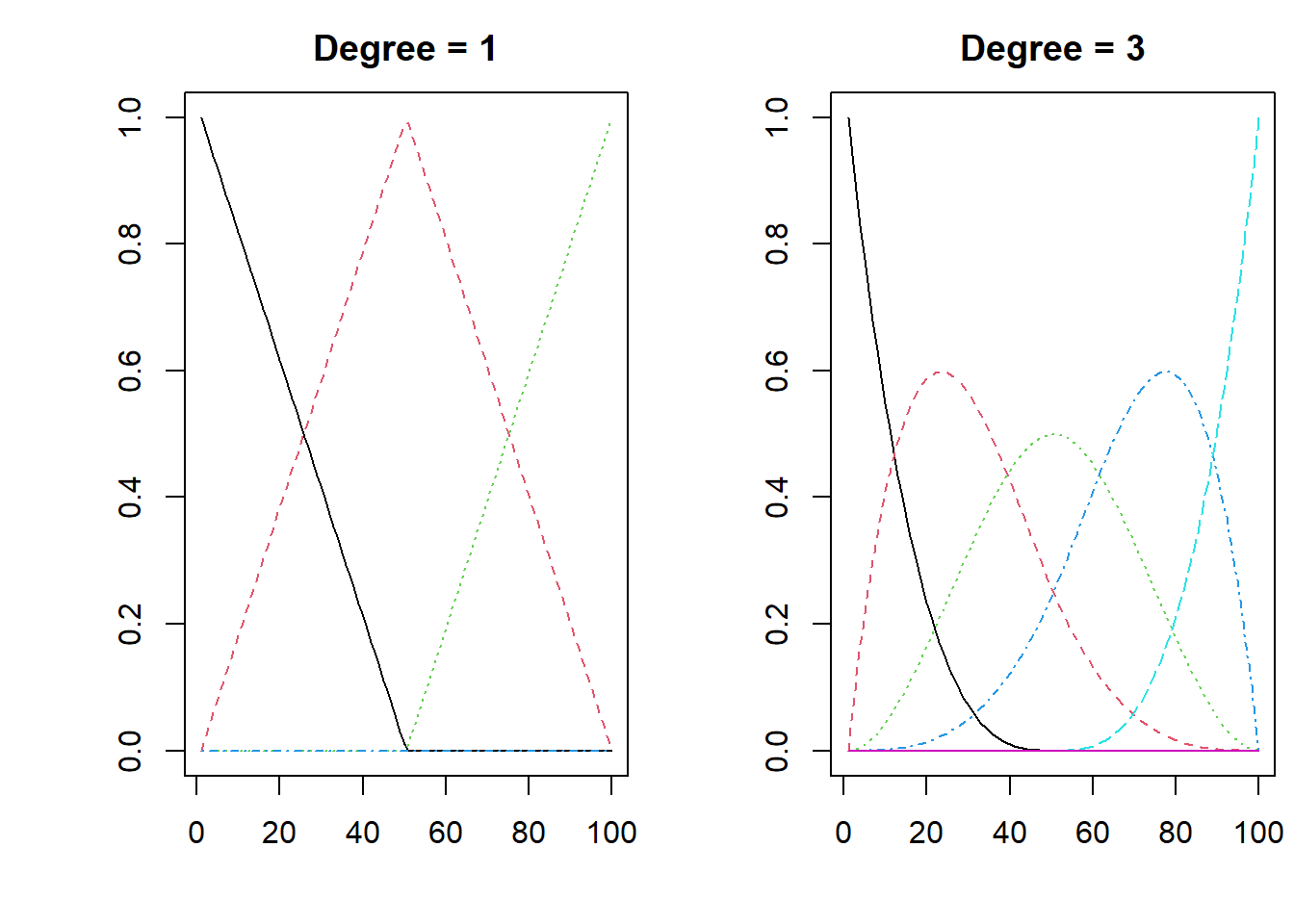
Figure 6.1: The flexibility of a spline
When you are not interested in the estimates for a specific characteristic, fitting a spline for that characteristics can be a useful approach. Say, for example, the age of the house. There might be many patterns for this variable. In a NMV hedonic model application, we are not specifically interested in the coefficient estimate for house age. We need to control for the effect of house age so that we do not get biased estimates of the variables we are interested in, but the parameter estimates for house age are not of interest. If we fit a spline to the house age characteristic. The model will then follow the pattern in the data for house age, whatever that pattern is, and we focus on the specific characteristics that we are interested in.
6.2.6 The median estimator as a robustness check
The main method of estimation used for hedonic price studies is the method of least squares. The method involves fitting a model to the data to minimise the sum of the squared error terms.
\[\begin{equation} min\sum\hat{e}_{ijt}^{2} \end{equation}\]
With this approach the estimated coefficients describe impacts, on average. Often this is the most useful description.
Sometimes we may also wish to describe effects at the median. For example, with a skewed distribution on house prices there can be a substantial difference between the mean and median values. One way to present a complementary assessment is to solve the following complementary model and find the estimates that minimise the sum of the absolute value of the errors.
\[\begin{equation} min\sum\left|\hat{e}_{ijt}\right| \end{equation}\]
This is Least Absolute Deviation regression, and solving this problem the estimates describe effects at the median. This approach also generalises to any quantile, but here we focus on the median as a robustness check on our main model findings. Note that minimising the sum of the square the errors implicitly places a large weight on large errors and this means that sometimes a small number of observations might pull the overall results in a specific direction. Minimising the sum of the absolute value of the error terms also protects against this.
For hypothesis testing median regression does not make the assumption of homoscedasity, and the the way the standard errors are calculated (via a bootstap method) naturally accounts for the variation in the data.
6.3 Worked example: Hedonic price regression
The steps in the process will be to:
- Read the data in the R from a spread sheer and check the data
- Visually explore the data as a sense check
- Estimate, test, and compare OLS models
- Conduct some robustness checks using other model types
This data is based on the Housing data set in the Ecdat package, although it has been extended.
The name of the data set is housingdata.new and the variables in the data set are:
- price = sale price of a house
- lotsize = the lot size of a property in square feet
- bedrooms = the number of bedrooms
- bathrms = the number of full bathrooms
- stories = the number of stories excluding basement
- airco = does the house has central air conditioning
- garagepl = the number of garage places
- prefarea = is the house located in designated close to green area parkland
- region = a spatial identifier (fixed effect) for the specific region
- time = a time of sale identifier (fixed effect) for year of sale
The data is read in and checked as followsL the command str(housingdata.new).
## 'data.frame':    4914 obs. of  10 variables:
##  $ price   : num  42000 38500 49500 60500 61000 66000 66000 69000 83800 88500 ...
##  $ lotsize : num  5850 4000 3060 6650 6360 4160 3880 4160 4800 5500 ...
##  $ bedrooms: num  3 2 3 3 2 3 3 3 3 3 ...
##  $ bathrms : num  1 1 1 1 1 1 2 1 1 2 ...
##  $ stories : num  2 1 1 2 1 1 2 3 1 4 ...
##  $ airco   : Factor w/ 2 levels "no","yes": 1 1 1 1 1 2 1 1 1 2 ...
##  $ garagepl: num  1 0 0 0 0 0 2 0 0 1 ...
##  $ prefarea: Factor w/ 2 levels "no","yes": 1 1 1 1 1 1 1 1 1 1 ...
##  $ region  : Factor w/ 3 levels "SA1","SA2","SA3": 1 1 1 1 1 1 1 1 1 1 ...
##  $ time    : Factor w/ 3 levels "2000","2001",..: 1 1 1 1 1 1 1 1 1 1 ...
Next we check the variables in the dataset to make sure they make sense. We look at the max and min values for each variable and the distribution across the quartiles to look for obvious errors, or other strange features in the data. With house price data there can be some extreme values
##      price           lotsize         bedrooms       bathrms        stories
##  Min.   : 16985   Min.   : 1650   Min.   :1.00   Min.   :1.00   Min.   :1.00
##  1st Qu.: 53636   1st Qu.: 3600   1st Qu.:2.00   1st Qu.:1.00   1st Qu.:1.00
##  Median : 70000   Median : 4600   Median :3.00   Median :1.00   Median :2.00
##  Mean   : 74523   Mean   : 5150   Mean   :2.97   Mean   :1.29   Mean   :1.81
##  3rd Qu.: 90000   3rd Qu.: 6360   3rd Qu.:3.00   3rd Qu.:2.00   3rd Qu.:2.00
##  Max.   :215293   Max.   :16200   Max.   :6.00   Max.   :4.00   Max.   :4.00
##  airco         garagepl     prefarea   region       time
##  no :3357   Min.   :0.000   no :3762   SA1:1638   2000:1638
##  yes:1557   1st Qu.:0.000   yes:1152   SA2:1638   2001:1638
##             Median :0.000              SA3:1638   2002:1638
##             Mean   :0.692
##             3rd Qu.:1.000
##             Max.   :3.000
Across the variables there is nothing that stands out as extreme. Note that there is not a great difference between the mean and median house price, so there may not be a great deal of difference between the mean and median model results.
It can be practical to exclide some observations from the data. For example, there maybe some very low sale prices recorded. These could be for houses that are related party transactions such as a transfer to another family member at a price below the market price; or they could be for houses that are very exclusive. From a statistical point of view, such property transactions represent transaction that are not part of the relevant population, and such properties should be excluded from the analysis. It is also possible that you may wish to specifically define the target population, for example only freestanding homes that include land. If that is the case, then you would want to restrict the sample to only free standing homes.
# To trim the top and bottom 1 percent of observations
housingdata.new1 <- quantile(housingdata.new$price, c(.01, .99))

# To define the target population and limit specific characteristics
housingdata.new1 <-subset(housingdata.new, price >=20000 & price<=200000 &
                region=="SA1" & garaepl<=5  & stories <=3 & bedroomrooms <=10)
The key variable we are interested in is the prefarea variable. This variable will ultimately provide an estimate of the value of being located in the preferred area, which in this application we define as being in close proximity to green space.
6.3.1 Visual data exploration
Confident that the data has been read in correctly, errors have been removed and or corrected, and the target population has been defined appropriately, we now explore the data visually.
Boxplots are effective for looking at some aspects of the data. Here we can see that, without controlling for other factors, house prices generally:
- increase with the number of bedroom, but maybe there is something different about houses with six bedrooms
- have higher sale prices in the preferred area close to green space
- vary in price spatially across the small area regions
- appear to have increased in price above inflation, through time.
boxplot(price~as.factor(bedrooms),las =1, col="grey", outcol ="grey",
        ylab = "", xlab = "Number of bedroom",
        main = "Price and bedrooms", horizontal =F,
        data = housingdata.new)

boxplot(price~as.factor(prefarea),las =1, col="grey", outcol ="grey",
        ylab = "", xlab = "Price",boxwex =0.6,
        main = "Price and green zone", horizontal =F,
        data = housingdata.new)

boxplot(price~region,las =1, col="grey", outcol ="grey",
        ylab = "", xlab = "Price",  boxwex =0.6,
        main = "Price and region fixed effect", horizontal =F,
        data = housingdata.new)

boxplot(price~time,las =1, col="grey", outcol ="grey",
        ylab = "", xlab = "Price", boxwex =0.6,
        main = "Price and time fixed effect", horizontal =F,
        data = housingdata.new)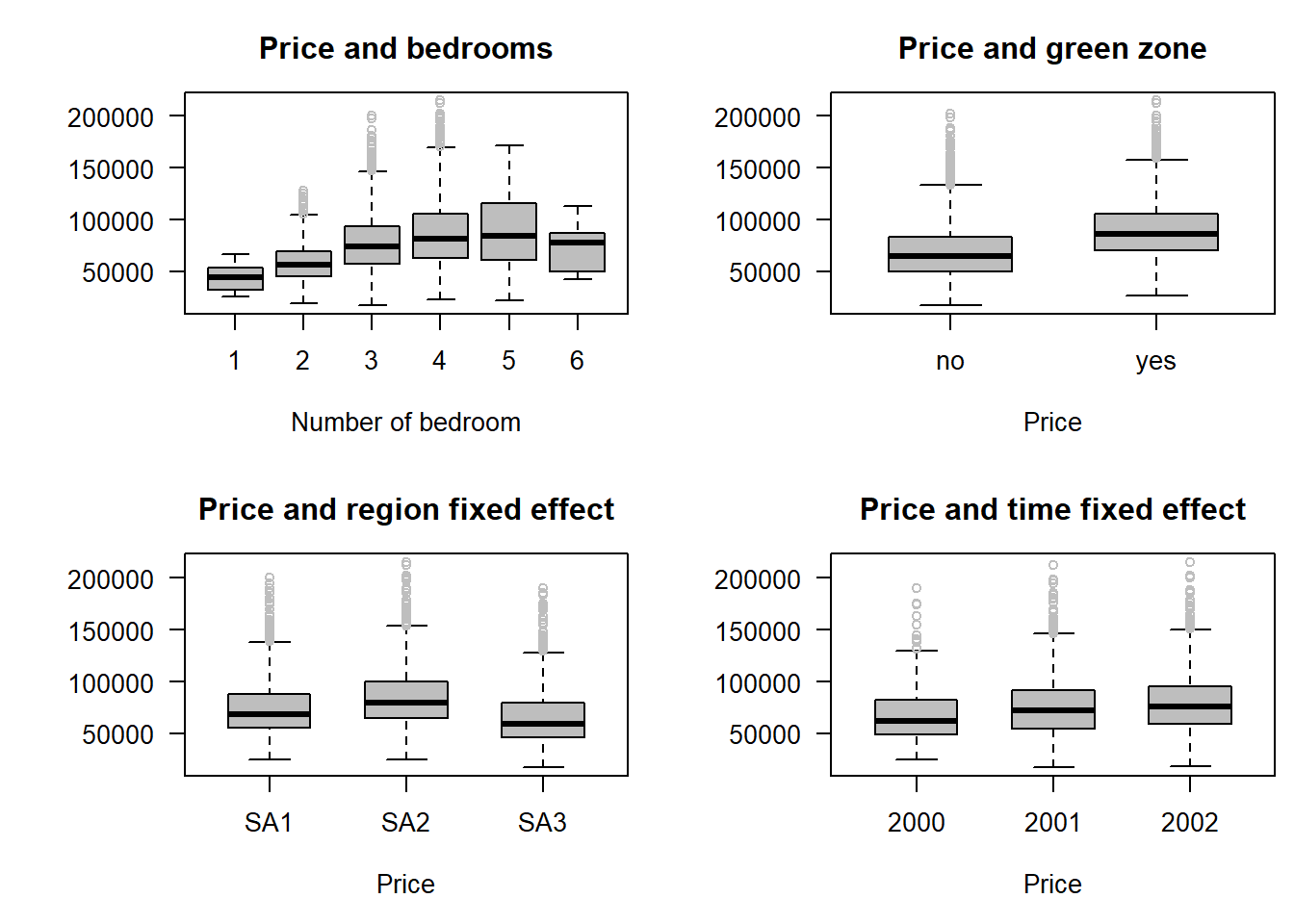
Figure 6.2: Exploring the impact of different housing attributes
It is also possible to look at the relationship between continuous variables. Here log house price is plotted on the y-axis, and log lot size is plotted on the x-axis. Additionally, the small area region is also identified. Overall there is a general positive relationship between log lot size and log price. It also looks as if houses with the same lot size sell for the least in SA3, and sell for the most in SA2, but there is also much variation.
plot(log(price)~log(lotsize), las=1,
     col= c(1:3 )[as.numeric(region)],
     #col= c("grey10","grey50","grey70" )[as.numeric(region)],
     #pch= c(1:3),
     xlab = "Log Lot Size (square feet)", ylab = "Log House Price",
     main = "",
     data = housingdata.new)

legend("topleft",
       title= "Lot size",
       legend= c("SA1","SA2","SA3" ),
       col=c(1:3),
       #col= c("grey10", "grey50","grey70" ),
       pch= c(1,1,1),
       bty="n")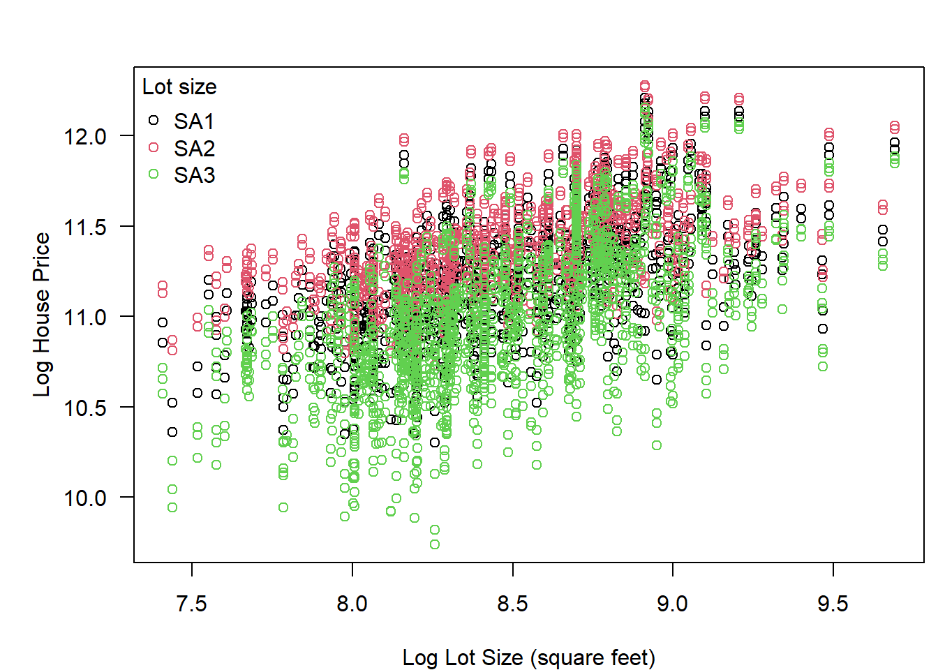
Figure 6.3: Exploring relationship between lot size and house price
6.3.2 Estimate and compare models
First, let us estimate the simple model, with a set of controls, and run the boxcox test to see what kind of transformation this test suggests for the response variable. A transformation of 1 is no transformation and a transformation of zero is a log transformation. The test says that the optimal transformation on the dependent variable is approximately a square root transformation.
Although it is possible to work with the square-root transformation, here we will (i) use the log-linear model as our base model; (ii) estimate the linear-linear model as a robustness check; estimate the LAD model as a further result robustness check.
lm.linear <- lm(price~lotsize+bedrooms+bathrms+stories+airco+garagepl+prefarea, data =housingdata.new)
boxcox(lm.linear)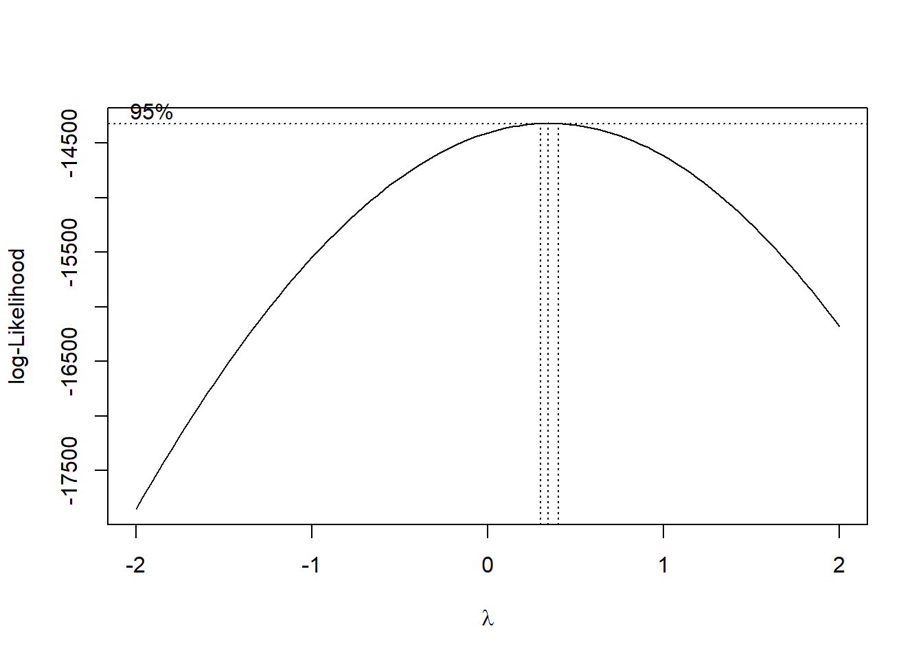
Now let us now estimate the:
Model 1. base model (just house characteristics)
Model 2. time fixed effects model
Model 3. spatial fixed effect model
Model 4. spatial and time fixed effects model.
Recall that Model 4 is the model that protects against omitted variables bias. The expectation is that estimates from this model are unbiased and consistent. In most applications the fixed effects in Model 4 consume many degrees of freedom. The more degrees of freedom the model ‘consumes’, other factors constant, the larger the standard errors. Adding variables that are not needed also results is an including irrelevant variables problem that results in the inflation of standard errors. With large standard errors the chance of a Type-II error (truth is that there is a difference and we fail to detect that difference) increases. So, if a smaller model is consistent with the data, we prefer the smaller model, as the smller model has greater power to detect a statistical difference, if truth is that there is a statistical difference to detect.
Following estimation models are compared using the anova function to implement an F-test. The way the tests are implemented in R means that the result can be seen as a test of whether the fixed effects are jointly statistically significant ie whether or not the fixed effects are needed for the model. In each case the test is framed as a comparison between a full model and a restricted model.
When the p-value from the anova F-test is less than 0.05, the conclusion drawn is that the more complete model (i.e. the model with fixed effects) results in a statistically significant improvement in model fit: hence the fixed effects are needed. When the test p-value is greater than 0.05, the conclusion drawn is that the more complete model (i.e. the model with fixed effects) does not results in a statistically significant improvement in model fit: the fixed effects are NOT needed, and we use the simpler model, without the fixed effect.
Normal practice is to start with the largest model and see if you can make it smaller. Here a full range of comparisons are shown for illustration purposes.
The first comparison shown is the comparison of the simple model the the model with time fixed effects: anova(lm.1,lm.t). As \(p<0.001\) the conclusion drawn is that the time fixed effects are jointly statistically significant and should be included in the model.
The second comparison shown is the comparison of the simple model the the model with spatial fixed effects: anova(lm.1,lm.s). As \(p<0.001\) the conclusion drawn is that the spatial fixed effects are jointly statistically significant and should be included in the model.
Comparisons are then show for the model with time fixed effects only compared to the model with both time and spatial fixed effects anova(lm.t,lm.st) and for the model with spatial fixed effects only compared to the model with both time and spatial fixed effects anova(lm.s,lm.st). For both these comparisons the model with both time and spatial fixed effects is a statistically better fit to the data.
Based on these comparisons, we continue the analysis with the time and spatial fixed effects model: this is the smallest model consistent with the data.
lm.1 <- lm(log(price)~lotsize+bedrooms+bathrms+stories+airco+garagepl+prefarea, data =housingdata.new)
lm.t <- lm(log(price)~lotsize+bedrooms+bathrms+stories+airco+garagepl+prefarea+time, data =housingdata.new)
lm.s <- lm(log(price)~lotsize+bedrooms+bathrms+stories+airco+garagepl+prefarea +region, data =housingdata.new)
lm.st <- lm(log(price)~lotsize+bedrooms+bathrms+stories+airco+garagepl+prefarea+ time+region, data =housingdata.new)

anova(lm.1,lm.t)
## Analysis of Variance Table
##
## Model 1: log(price) ~ lotsize + bedrooms + bathrms + stories + airco +
## garagepl + prefarea
## Model 2: log(price) ~ lotsize + bedrooms + bathrms + stories + airco +
## garagepl + prefarea + time
## Res.Df RSS Df Sum of Sq F Pr(>F)
## 1 4906 351.7
## 2 4904 329.9 2 21.77 161.8 <2e-16 ***
## ---
## Signif. codes: 0 '***' 0.001 '**' 0.01 '*' 0.05 '.' 0.1 ' ' 1## Analysis of Variance Table
##
## Model 1: log(price) ~ lotsize + bedrooms + bathrms + stories + airco +
## garagepl + prefarea
## Model 2: log(price) ~ lotsize + bedrooms + bathrms + stories + airco +
## garagepl + prefarea + region
## Res.Df RSS Df Sum of Sq F Pr(>F)
## 1 4906 351.7
## 2 4904 287.1 2 64.55 551.3 <2e-16 ***
## ---
## Signif. codes: 0 '***' 0.001 '**' 0.01 '*' 0.05 '.' 0.1 ' ' 1## Analysis of Variance Table
##
## Model 1: log(price) ~ lotsize + bedrooms + bathrms + stories + airco +
## garagepl + prefarea + time
## Model 2: log(price) ~ lotsize + bedrooms + bathrms + stories + airco +
## garagepl + prefarea + time + region
## Res.Df RSS Df Sum of Sq F Pr(>F)
## 1 4904 329.9
## 2 4902 265.3 2 64.55 596.3 <2e-16 ***
## ---
## Signif. codes: 0 '***' 0.001 '**' 0.01 '*' 0.05 '.' 0.1 ' ' 1## Analysis of Variance Table
##
## Model 1: log(price) ~ lotsize + bedrooms + bathrms + stories + airco +
## garagepl + prefarea + region
## Model 2: log(price) ~ lotsize + bedrooms + bathrms + stories + airco +
## garagepl + prefarea + time + region
## Res.Df RSS Df Sum of Sq F Pr(>F)
## 1 4904 287.1
## 2 4902 265.3 2 21.77 201.1 <2e-16 ***
## ---
## Signif. codes: 0 '***' 0.001 '**' 0.01 '*' 0.05 '.' 0.1 ' ' 16.3.2.1 Adjust standard errors
For inference it is almost always the case that heteroskedasticty will be an issue. Here we formally test for heteroskedasticty. Low p-values are evidence agaist the null of no heteroskedasticty. The bptest is in the MASS package, which is loaded with AER.
##
##  studentized Breusch-Pagan test
##
## data:  lm.st
## BP = 283.5, df = 11, p-value <2e-16
As \(p<0.001\) we reject the null of homoskedastic errors, and apply robust standard errors.
You can get the robust SE values using the following call as a general approach, where the sandwich package has been loaded with AER.
The core model results, and robust standard errors can be integrated into a single results table as follows:
V <- vcovHC(lm.st)
sumry <- summary(lm.st)
table <- coef(sumry)
table[,2] <- sqrt(diag(V))
table[,3] <- table[,1]/table[,2]
table[,4] <- 2*pt(abs(table[,3]), df.residual(lm.st), lower.tail=FALSE)
sumry$coefficients <- table
print(sumry)
The particular estimate of interest is the estimate associated with the prefareyes variable. This is the coefficient that describes the average impact on house prices of being with the boundary of what has been defined as close to greenspace.
##              Estimate Std. Error t value     Pr(>|t|)
## garagepl    0.0569288 0.00433572 13.1302  9.89224e-39
## prefareayes 0.1597272 0.00698932 22.8530 6.31401e-110
## time2001    0.1025501 0.00844918 12.1373  2.01288e-33
% Error: Unrecognized object type. % Error: Unrecognized object type. % Error: Unrecognized object type. % Error: Unrecognized object type.
Recall the formula for the dummy variable for close to greenspace when there is a log transformation on the dependent variable is :\(100\times exp[\beta_{k}]-1\).
So we have = \(100\times exp[0.16]-1= 17.3\) percent as the estimate of the average increase in house prices, for being close to greenspace, other factors held constant.
It is also good practice to report the 95 percent confidence interval for the estimate. For large data sets this will generally be \(\beta_{k}\pm 1.96\times SE_{\beta_k}\), and for this example, as \(SE_{\beta_k} =0.007\) the 95 percent confidence interval is \([15.7\% - 18.9\%]\).
You can also report the effect in dollar value terms. The average house price in the sample data is $74,523 and applying the percentage change estimates to the average house price, the central estimate of value is $ 12,893 with 95 percent confidence interval [$11,700 to $14,085].
6.3.2.2 A spline for a variable
Here we fit a spline to the bedrooms variable. This just means that we say, let the data fit the pattern for bedrooms in some general flexible manner, because we have no theory for how price should be related to bedrooms. The study focus is the prefarea variable so adding this flexibility for bedrooms does not detract from estimating the impact of the variable of interest. To fit the spline to the bedrooms variable load the splines package and then wrap the relevant variable as follows bs(bedrooms).
The summary() function and coeftest(lm.spline,vcovHC(lm.spline)) can be used to look at the results.
lm.spline <- lm(log(price)~lotsize+bs(bedrooms)+bathrms+stories+airco+garagepl+prefarea+ time+region, data =housingdata.new)

coeftest(lm.spline,vcovHC(lm.spline))
##
## t test of coefficients:
##
## Estimate Std. Error t value Pr(>|t|)
## (Intercept) 1.006e+01 3.454e-02 291.314 < 2e-16 ***
## lotsize 5.133e-05 1.748e-06 29.360 < 2e-16 ***
## bs(bedrooms)1 4.817e-01 8.048e-02 5.986 2.3e-09 ***
## bs(bedrooms)2 1.107e-01 4.038e-02 2.741 0.00614 **
## bs(bedrooms)3 3.667e-01 6.452e-02 5.684 1.4e-08 ***
## bathrms 1.796e-01 8.037e-03 22.342 < 2e-16 ***
## stories 7.382e-02 3.799e-03 19.434 < 2e-16 ***
## aircoyes 1.646e-01 7.402e-03 22.241 < 2e-16 ***
## garagepl 5.577e-02 4.327e-03 12.888 < 2e-16 ***
## prefareayes 1.536e-01 7.123e-03 21.565 < 2e-16 ***
## time2001 1.026e-01 8.426e-03 12.171 < 2e-16 ***
## time2002 1.610e-01 8.221e-03 19.588 < 2e-16 ***
## regionSA2 1.333e-01 7.444e-03 17.907 < 2e-16 ***
## regionSA3 -1.473e-01 8.373e-03 -17.595 < 2e-16 ***
## ---
## Signif. codes: 0 '***' 0.001 '**' 0.01 '*' 0.05 '.' 0.1 ' ' 1Note that the terms on bedrooms are all significant, and so the impact of extra bedrooms appears to follow a pattern more complex than allowed for in the standard model. The estimate for the prefarea variable is, however, little changed by adding this extra flexibility to the model: 0.154 for the spline model compared to 0.16 for the original model.
6.3.2.3 LAD estimator
Here we solve for the conditional median, rather than the conditional mean, using the quantreg package. This can be seen as a good robustness check on the core results. For the conditional median, we also solve for the median house price not the mean house price.
lm.median <- rq(log(price)~lotsize+bedrooms+bathrms+stories+airco+garagepl+prefarea+ time+region, data =housingdata.new,tau = 0.5 )
#  Just show the relevant section of the output
summary(lm.median)$coefficients[7:9,]
## Value Std. Error t value Pr(>|t|)
## garagepl 0.0427122 0.00393097 10.8656 0
## prefareayes 0.1661073 0.00628217 26.4411 0
## time2001 0.1093518 0.00808509 13.5251 0The estimate is again similar to the original result, with the median model estimate 0.166 compared to 0.16 for the original model.
6.3.2.4 A model with no transformation on the dependent variable
Finally, we also estimate a model with price untransformed as the dependent variable, and look at the estimates across the different models. We are looking for consistency in the results. Recall that the box-cox transformation suggested that the theoretical ideal model was likely to be somewhere inbetween the log model and the no transformation model.
This model says the
lm.linear <- lm(price~lotsize+bedrooms+bathrms+stories+airco+garagepl+prefarea+ time+region, data =housingdata.new)

# Test for heteroskedasticty
bptest(lm.linear)

# As the model fails the heteroskedasticty, use robust standard errors
coeftest(lm.linear,vcovHC(lm.linear))

#  Just show the relevant section of the output
summary(lm.median)$coefficients[7:9,]
## Estimate Std. Error t value Pr(>|t|)
## garagepl 4829.31 351.158 13.7525 2.96792e-42
## prefareayes 11728.05 600.675 19.5248 8.07627e-82
## time2001 7611.08 603.429 12.6130 6.43300e-36Again the result for the model with price untransformed as the dependent variable $ 11,728 is similar to the original model result, when expressed in dollars at the sample mean house price $12,893 for the original model.
6.3.3 Comparing model results
It is good practice to report the results from the different models estimated. Here all four model results are shown. In this instance, across all models the estimate of the value capitalised into house prices of being close to public open space coefficient is stable, and the standard error relatively small.
To put the results in perspective, the percentage change estimates are evaluated at the sample mean values for the spline and log-linear model to get dollar values. For the linear model the base estimate is on the dollar scale. For the median model the percentage change is evaluated at the median house price, as this also presents a comparison result.
For our base case model the estimated impact of being close to greenspace, evaluated at the mean house price, is $12,893; when we fit a partial linear model using spline functions for the effect of additional bedrooms, the estimated impact of being close to greenspace is $12,371; when we fit the model as a linear model with price rather than log price the estimated impact of being close to greenspace is $11,728; and when we estimate a median model the estimated impact of being close to greenspace is $12,670.
| Regression Model | Est ($) | 95%-Low ($) | 95%-Hi ($) |
|---|---|---|---|
| Log-linear base model | 12,893 | 11,700 | 14,085 |
| Log-linear spline model | 12,371 | 11,179 | 13,563 |
| Log-linear median model | 12,670 | 11,620 | 13,650 |
| Linear-linear model | 11,728 | 10,551 | 12,905 |
That all the models estimated provide similar results suggests that the finding is robust. Based on these results, you might might say that the value of being close to greenspace is an increase in house price values of around $11,500, or between $11,000 and $12,000.
This value can then be used in public policy discussions and cost-benefit analysis.